Maps! Maps! Maps!

The ggmap package is awesome. It enables you to get a map from Google maps (in various forms too! Just check out the package documentation) and then you can plot stuff on top of the maps, which is really useful particularly if you are dealing with spatial data.

# Load in the package
library(ggmap)

# Get a map!
# For fun, I'll do my home town. ggmap does surprisingly well with 
# limited search terms, so you do not have to worry about being super # specific or explicit. 
map <- get_map(location = 'Soda Bay,
               California', zoom = 11)

# The 'base' of this is ggmap(map). This will just 'print' your map. 
ggmap(map)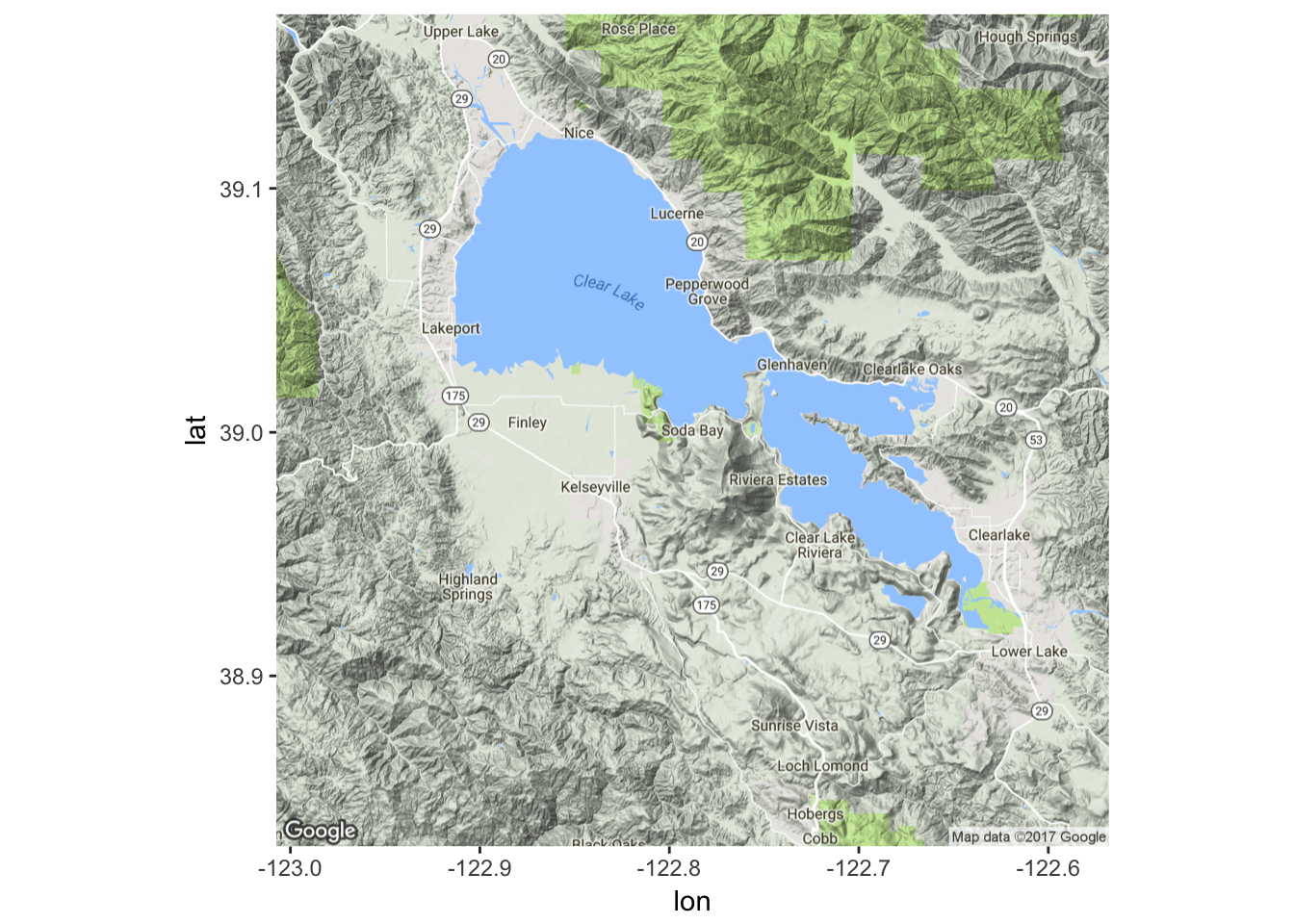

Now you can use ggplot2 to plot stuff on top of the map you’ve just generated. This is useful for all kinds of spatial data, like geotagged social media posts or census data. Here’s an example with census data. (If you want to see how I got this data with R, check out this post here or this tutorial here or here or here!)

ggmap(map) +
  geom_polygon(data = homevalue_points, aes(x = long, y = lat, group = group, fill = Median_Value),   alpha=0.75) +
  scale_fill_distiller(palette = "Blues") +
  guides(fill = guide_legend(reverse = TRUE)) +
  theme_nothing(legend=TRUE) +
  coord_map() +
  labs(title = "2013 Median Value for Owner-Occupied Housing Units",
  fill = "Value (Dollars)")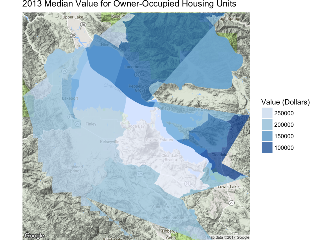

In essence, think of the ggmap as a base which you can build on. As long as you have coordinates, you are able to plot things on top of a ggmap, even series of data!