Intro to R and R Studio
The term ‘R’ refers to both a programming language and the environment in which you execute commands and manipulate data. R is a command-line interface, which means you tell R what you want it to do via lines of text. Most commands you will be using will come from different packages people have developed for R – this means that when you issue a command, you are often actually invoking a series of commands someone has encoded in the command you are using. There are other more basic commands in R you can use without downloading and loading packages, so we will start there to get a sense of how the command-line works.
R is a language – it has syntactic rules, preferred word order and both required and optional arguments in each command you issue. Let’s start with setting our current working directory. A directory is the ‘location’ of where your data is currently being drawn from and/or saved to. Check the location of your current working directory with the following command:
getwd()## [1] "/Users/katelyons/katelyons/content/portfolio"If this is where your data is, or where you’d like to save things, great! If not, you can change your working directory. The argument you will put for this command is the path of the directory you want to use. You can see what most of your path will look like from the results of getwd() – just adjust it to the specific folder you want to work in. The one I’ve put as an example is for my computer – yours (especially if you are not using a Mac!) will look different:
# setwd("/Users/katelyons/Documents/Workshop")This is a fundamental lesson about R – you have to be careful to be specific and when you get an error, make sure to think about what you are telling R to do in each command. Often you’ll find an error is just leaving a parentheses out or forgetting that something needs to be in quotes! (For example, when writing this I forgot to add the “” around my path and got an error!)
A great resource to look at command syntax and arguments is R help. You can either use the ‘Help’ tab in R Studio and type in the command in the search field, or use the command-line:
# ?getwd()Another important thing to think about and remember about R are the different data types and objects that you can work with in this environment. ‘Data type’ refers to, in a loose way, the format or form of your data. What type your data is represented by influences what kind of commands you can use to manipulate the data. You’ll mainly encounter three types of types in our work on text and social media mining: character, factor and logical. This collection of slides provides a nice summary of definitions and examples that I will reproduce here. They label these types in terms of ‘vectors’. Vectors are “sequence[s] of data elements of the same basic type” (see here) – so just a way of describing more than one instance of these representations of your data.
- Character or string vector: “each element in the vector is a string of one or more characters”
# Let's make a character vector
char_vector <- c("this", "is", "a", "character", "vector")
# This command says concatenate (the little c) the following series of strings of characters that are encapsulated in the parentheses and put that concatenated result into (the '<-') a value that I will call 'char_vector'.

# You can use R to evaluate different aspects of character vectors like number of strings, numbers of characters in each string or whether or not a string is present in your vector

# How many strings does my vector have?
length(char_vector)
## [1] 5# How many characters are in each string?
nchar(char_vector)## [1] 4 2 1 9 6# Which string matches 'a'?
char_vector == "a"## [1] FALSE FALSE TRUE FALSE FALSE# Note use of double equals signs. We do this because '=' is another way to perform '<-'. So we had run char_vector = "a" the vector would have changed to the character "a". This wouldn't be the end of the world, because we could go back and re-create the original character vector again. R does not have an 'un-do' however, so be careful about accidentally overwriting something you do not want to overwrite. A good practice to avoid this is if you are trying a command out, just create a new output value. We'll see more examples of this practice as we perform more complex commands.
char_vector2 <- c("this", "is", "a", "test")- Logical: “binary, two values represented by TRUE and FALSE”
# We've already been introduced to this value in the previous example. We can store the output of our char_value == 'a' command in a new value, which will be a vector of logical types!
logical_vector <- char_vector == "a"

#Check it out
logical_vector
## [1] FALSE FALSE TRUE FALSE FALSE- Factor: “set of numeric codes with character-valued levels”
# I've adapted this example from the statistics slides. Here we have a subset of sharks we are studying, consisting of four great white sharks and two mako sharks.
sharks = factor(c(1,0,1,0,0,0), levels = c(0, 1), labels = c("great_white", "mako"))
# Note how I've used '=' instead of '<-'. It really doesn't matter which one you use. The same holds for ' vs. ". " can be easier because R Studio will automatically provide the accompanying quotation mark (helping you not forgetting it and avoiding a syntax error).
# This command says concatenate a factor of two occurances of 1 and four occurances of 0, the two different levels of this factor are 0 and 1 and these values will be named respectively 'great_white' and 'mako'. Note that the label has to be one string -- so a two word phrase like 'great white' has to be 'great_white'.
You can check what kind of vector you are working with with the class command.
class(char_vector)## [1] "character"class(logical_vector)## [1] "logical"class(sharks)## [1] "factor"Now we understand what a vector is, let’s more to more complicated representations of data. From stats slides:
- Vector: “a collection of ordered homogeneous elements”
- “We can think of matrices, arrays, lists and data frames as deviations from a vector”
We won’t go into matrices, arrays or lists because we won’t be working with any of those things, but we WILL be working with data frames:
- Data Frame: “a list with possible heterogeneous vector elements of the same length. The elements of a data frame can be numeric vectors, factor vectors, and logical vectors, but they must all be of the same length” (emphasis added)
shark_id = c(1, 7, 4, 2)
species = c("great_white", "whale", "mako", "hammerhead")
sex = c("f", "m", "f", "f")
shark_df = data.frame(shark_id, species, sex)
# You can also see if something is a data frame using class
class(shark_df)
## [1] "data.frame"# For data frames we can either use the 'View' command to open it in a different window (useful for larger data frames) or 'head' to see the first few entries in the data frame (also useful for larger data frames). Because our data frame is so small, we can also just type in the name to see the entire thing
shark_df## shark_id species sex
## 1 1 great_white f
## 2 7 whale m
## 3 4 mako f
## 4 2 hammerhead fWe can learn a lot about our data frame with some other commands:
# What are all the vectors in our data frame? We could also think of this as 'what categories are in my data frame'?
names(shark_df)
## [1] "shark_id" "species" "sex"# How many categories? (Helpful for large data frames)
length(shark_df)## [1] 3# What levels are present in a category?
levels(shark_df$species)## [1] "great_white" "hammerhead" "mako" "whale"# This last command introduces the '$' -- this just singles out a particular column or category. For some commands you need to be specific as to which column in the data frame you are referring to, as in this case. We can't ask R to tell us the levels of the entire data frame because that wouldn't make sense to R -- where would it look? How would it know that you meant 'for each column tell me the levels' -- the 'levels' command just tells R 'tell me the different levels in this category' so you have to specify which category. <- Hopefully this is insightful into the fundamental 'sense' of how to use R: be specific and try to think about what the command is telling R to do. This is really helpful when you run into errors, which you most certainly WILL do.
# We can get a more general sense of our data frame too
summary(shark_df)## shark_id species sex
## Min. :1.00 great_white:1 f:3
## 1st Qu.:1.75 hammerhead :1 m:1
## Median :3.00 mako :1
## Mean :3.50 whale :1
## 3rd Qu.:4.75
## Max. :7.00Interesting! Do you see how it treated ‘shark_id’ like numeric values? That isn’t what we meant! But of course R would think that because it makes the most sense to R – numbers are treated as numbers, the first assumption is not to treat these numbers as symbols for something else! Luckily, however, most of the time it is easy to straighten this out by telling R you want to treat a category ‘as’ something – in this case, ‘as.factor’:
# Again, make sure you specify the column
# You also have to 'save' this transformation by 'putting' the result into the column of the data frame you are transforming. Otherwise, R just thinks 'oh, you want to see what this would look like if this column was a factor'
shark_df$shark_id <- as.factor(shark_df$shark_id)

# If we made a mistake and want to turn it into a number again, just use
# as.numeric(shark_df$shark_id)

# Let's try again
summary(shark_df)
## shark_id species sex
## 1:1 great_white:1 f:3
## 2:1 hammerhead :1 m:1
## 4:1 mako :1
## 7:1 whale :1You can think of data frames like an Excel or CSV (comma separated value) file. In fact, when you load in an excel or CSV, it automatically becomes a data frame. Let’s try this with some actual data, a CSV file of 50 subsetted tweets from my dissertation data.
# Make sure you are in the same directory as the location of the file you are trying to load in or R cannot find it
data2 <- read.csv("subtweets.csv", header=T)
# This is telling R, find a CSV file with this exact name and load it into my work space. It is also telling R that it is true that this file has a header with category names. If this was marked 'F' R would treat the first row as observations.
# CSV is basically the same as Excel, except CSV doesn't require a separate package in R to load it in. There are packages that can do this, but I prefer if I am working with something I created in Excel to just 'Save As' the file as CSV from the Excel side. This is just a personal preference.
# Check what class
class(data2)
## [1] "data.frame"# What does this data frame look like?
# View(data2)We will routinely be using R to load in and export out data, usually in CSV. Sometimes this can mess up the encoding of your data however (e.g. if you just downloaded tweets and haven’t tagged emojis yet, saving to CSV will lose the encoding) so if you are just saving something you are working on and want to come back later, you can save it as R data. This is a really helpful thing you can do, because it doesn’t matter what the object is (it can be a vector, list, data frame, etc.) and when you load it back it it’s just how you left it.
# When you want to save something you have been working on (this will automatically save it to your current working directory)
save(data2,file=paste("sampledata.Rda"))

# When you want to load it in (make sure you're in the same directory as where you saved this)
load('sampledata.Rda')
Now let’s look at this data and use some packages to do different things with it! This is a file of mined tweets. We have ‘document’, which is the number id of the tweet in the corpus; ‘text’ which is the content of the tweet; ‘favorited’ which is the number of times the tweet has been favorited; ‘created’, when the tweet was tweeted; ‘truncated’, ‘replytoSID’ which I have never needed so never researched what they are; ‘id’ which is Twitter’s in-house id # for the tweet and ‘replyToUID’, another thing I’ve never used; ‘statusSource’ which is all Instagram bc I just wanted to work with Instagram data; ‘screenName’ which is name of the poster; ‘retweetsCount’, how many times the tweet was re-tweeted; ‘isRetweet’, whether or not a tweet is a re-tweet of someone else and finally, ‘longitude’ and ‘latitude’, the coordinates of where the tweet has been geotagged by the user.
names(data2)## [1] "X" "document" "text" "favorited"
## [5] "favoriteCount" "replyToSN" "created" "truncated"
## [9] "replyToSID" "id" "replyToUID" "statusSource"
## [13] "screenName" "retweetCount" "isRetweet" "retweeted"
## [17] "longitude" "latitude"At least for this workshop, you’ll be working primarily with data frames (or spending time turning something into a data frame so can you can work with it). Data frames have a lot of useful features. For example, they are really easy to subset. For example, in my data set I had a number of spam posts that were generated by bots that weren’t informative to my research question. How do I get rid of those posts?
# Get rid of super frequent spam posters
# Note I'm creating a new data frame, data3 so I don't 'lose' my original data frame just yet
data3 <- data2[! data2$screenName %in% c("4AMSOUNDS",
      "BruciusTattoo","LionsHeartSF","hermesalchemist","Mrsourmash","AaronTheEra","AmnesiaBar","audreymose2","audreymosez","Bernalcutlery","blncdbrkfst","BrunosSF","chiddythekidd","ChurchChills","deeXiepoo","fabricoutletsf","gever","miramirasf","papalote415","HappyHoundsMasg","faern_me"),]

# Let's use another useful command called 'nrow' to check the number of rows and see how many posts got eliminated
nrow(data3)
## [1] 44The above command is an introduction to the wonderful world of regular expressions (regex. A lot of the packages we’ll be dealing with eliminate the need to use regular expressions, but we will still need them occasionally nonetheless. The most frustrating aspects of regex are the things that make them so powerful and useful. Regex use specific sets of commands made up of specific common symbols to describe ‘sets of strings’ (R Documentation). So, in this example above, we’ve used regex to say subset (the ‘[]’) everything in the data2$screenName column that is NOT (the ‘!’) present (the ‘%in%’) this list of values (‘c’ concatenate, then the list of names of posters you don’t want). (Technically ‘%in%’ isn’t a regex – it’s part of base R and used to ‘match’ values. There is a way to match using regex but %in% is much more intuitive). We could also use a modified version of this command to isolate those spam posters like so:
# Just remove the '!'
test <- data2[ data2$screenName %in% c("4AMSOUNDS",
      "BruciusTattoo","LionsHeartSF","hermesalchemist","Mrsourmash","AaronTheEra","AmnesiaBar","audreymose2","audreymosez","Bernalcutlery","blncdbrkfst","BrunosSF","chiddythekidd","ChurchChills","deeXiepoo","fabricoutletsf","gever","miramirasf","papalote415","HappyHoundsMasg","faern_me"),]

# View(test)
We’ll return to regex in the coming weeks, especially when we want to identify values that match a certain set of characteristics.
Now that we have some experience with the command line, let’s download and load some packages and use them to look at our data. I also want to introduce both the ggplot2 package itself as a visualization tool and introduce the logic of that package (which can often confuse and frustrate people working with it for the first time!).
When you want to use a package in R, you have to download the package AND load the package into your library. Once you download a package once, you won’t have to download it again (unless you upgrade R, sometimes you have to re-download to do that) but you will have to re-load it in your library whenever you’ve opened a new session. Let’s start with getting the ggplot2 package and the ggmap package.
# install.packages("tidyverse")
# This will not only give us ggplot2, but a whole other slew of packages that will be really useful down the line like dplyr, tidyr, purrr, etc.
# install.packages("ggmap")
library(tidyverse)
library(ggmap)
Now what we are going to do is use the ggmap package to download a map from Google Map’s API (Application Programming Interface – more about this in week 3) and plot the location of tweets using ggplot2. Let’s start with ggmap:
# Let's start with ggmap's 'get_map' function, which allows you to specify a location (depending on what you are looking at it this could be more vauge like 'San Francisco, California' or 'California')
# The 'zoom' parameter is just how close you want to be. For me, I was looking at a neighborhood so this is pretty close, but you can play around with it to get the map you want.
map <- get_map(location = 'Valencia St. and 20th, San Francisco, California', zoom = 15)

#Check out the map (it'll pop up in your 'Plots' tab in R Studio -- you can click 'Zoom' if you want a closer look)
ggmap(map)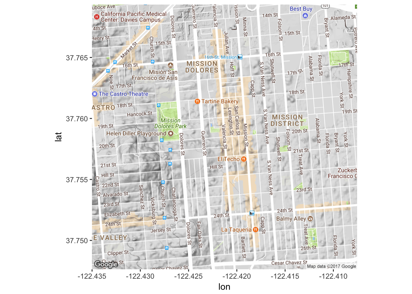
Great! We have our map. Now let’s plot stuff on it. The inherent idea behind ggplot2 is layering. You build a visualization (graph, map, etc.) layer by layer. So here we will tell ggplot2 that we want our map as a ground layer, with the coordinates of our tweets put on top of that. Luckily, ggmap maintains latitude and longitude so when we tell ggplot2 what our x and y axes are, they’ll match up with the ones on the map. As always, however, we will have to do some preliminary steps to make sure everything is in the right format.
data3$longitude<-as.numeric(data3$longitude)
data3$latitude<-as.numeric(data3$latitude)

mapPoints <- ggmap(map) + geom_point(aes(x = longitude, y = latitude),
                                     data=data3, alpha=0.5, size = 3)
mapPoints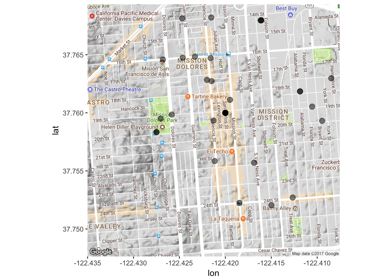
Great! What if we want to look at this from a bit further away? We’d have to change the map layer. So, we get another map.
map2 <- get_map(location = 'Valencia St. and 20th, San Francisco, California', zoom = 13)
ggmap(map2)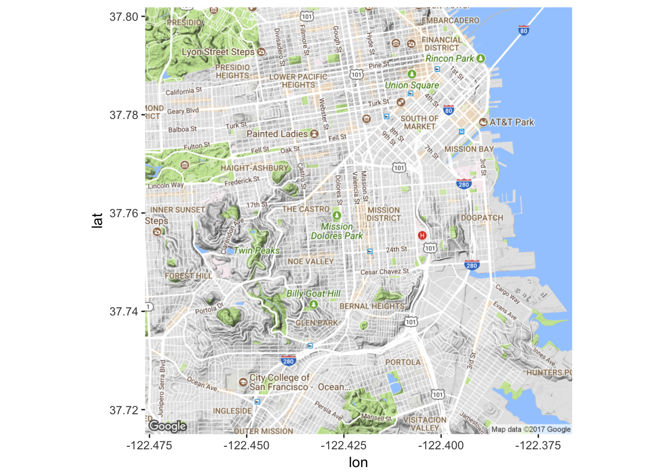
# Map it again!
mapPoints2 <- ggmap(map2) + geom_point(aes(x = longitude, y = latitude),
                                     data=data3, alpha=0.5, size = 3)
mapPoints2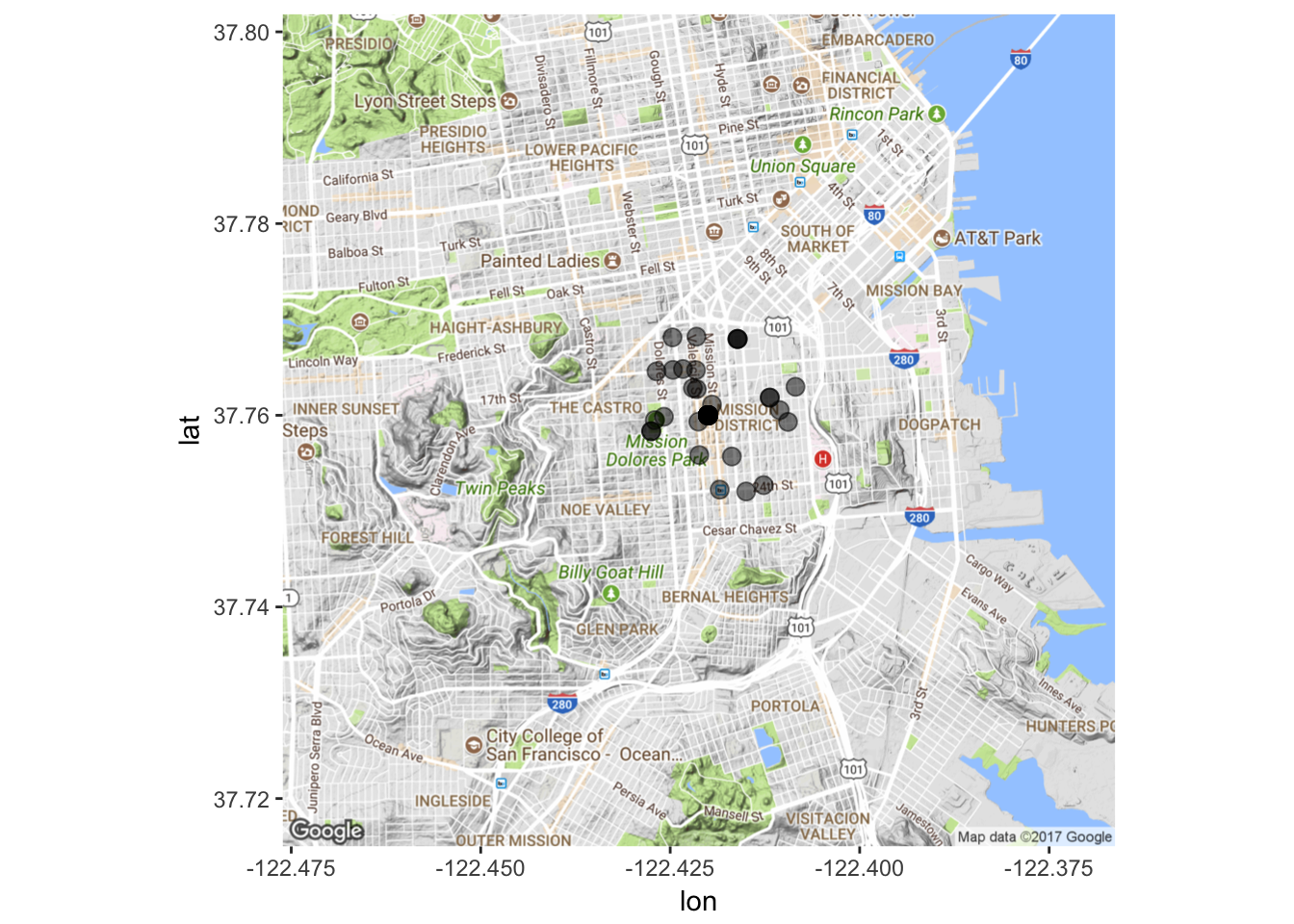
As we will see, we can encode lots of different information in maps other than just location, but this necessitates identifying other features we might want to showcase on our map. We don’t have any of those yet, but we can pretend screen name is one of those things.
# Note the only thing that changes is 'color'. This tells ggplot2 I want to distinguish each dot by differences in category 'screenName'
mapPoints3 <- ggmap(map) + geom_point(aes(x = longitude, y = latitude, color = screenName),
                                     data=data3, alpha=0.5, size = 3)
mapPoints3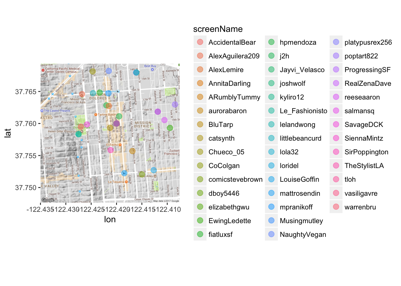
Gross! Too many names. Let’s first use the dplyr package to subset the data so it’s not TOO messy. Let’s pick a random 10 tweets.
# dplyr package is already loaded as part of the 'tidyverse'
submap <- sample_n(data3, 10)

# Note the only thing that changes is data to 'submap'
mapPoints4 <- ggmap(map) + geom_point(aes(x = longitude, y = latitude, color = screenName),
                                     data=submap, alpha=0.5, size = 3)
mapPoints4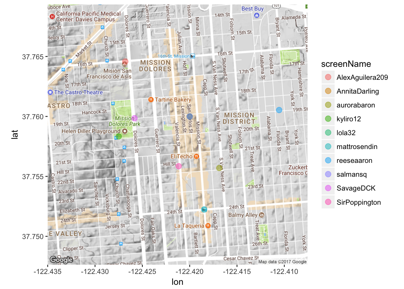
That’s kind of faint. Because I don’t have too much overlap, I’ll make the dots more opaque by playing around with the ‘alpha’ argument.
mapPoints5 <- ggmap(map) + geom_point(aes(x = longitude, y = latitude, color = screenName),
                                     data=submap, alpha=1, size = 3)
mapPoints5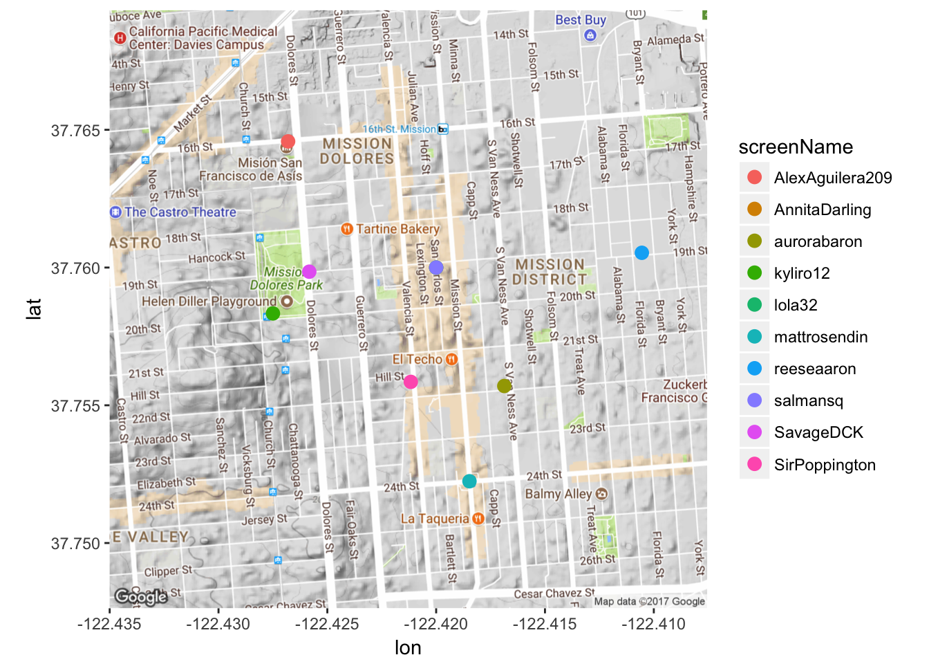
Next week: loading in, cleaning and playing around with text files!