Intro to Text Mining
There are many examples of doing analyses of texts in English, but not as many in other languages. To address this somewhat I’ll be looking at librettos of operas on stage at the Metropolitan Opera this season (2017-2018) as these have a lot of variation linguistically and also offer some unique and interesting processing challenges.
Let’s start with Mozart’s ‘Cosi Fan Tutte’ (libretto by Da Ponte).
To prepare this data, I copy-pasted it from the above site into Word and then saved it as a ‘.txt’ file. IMPORTANT: Because there are ‘special characters’ due to it’s being in Italian, I made sure to save it in UTF-8 encoding so those would be maintained in R. As a best practice, I’d recommend you save most text files you’ll be importing into R in this manner.
You can access the Cosi Fan Tutte data here.
# Make sure you have all the right packages
packs = c("stringr","ggplot2", "tm","wordcloud","plyr","tidytext","dplyr","tidyr", "readr")
# If you need to re-install (which you might have to if you got a new R Studio version) here is a shortcut:
# lapply(packs, install.packages, character.only=T)
lapply(packs, library, character.only=T)
# Set your directory
# setwd("/Users/katelyons/Documents/Workshop")
# library(devtools)
# This might be a nice way to work with data like this (or transcript data) but due to issues with rJava I'm not going to explore it now. If rJava works for you, this might be a package to check out!
# install_github("qdap", "trinker", depend)
# library(qdap)
# library(trinker)
# Each scene is saved as a separate text file so I have to load in each one and then combine them in R. We will use the readr package to read in each file
library(readr)
# Depending on where your file is you might need to include the entire path
# a1s1 <- readLines("cosi/a1s1.txt")
a1s1 <- readLines("cosi/a1s1.txt")
a1s2 <- readLines("cosi/a1s2.txt")
a1s2 <- readLines("cosi/a1s2.txt")
a1s3 <- readLines("cosi/a1s3.txt")
a1s4 <- readLines("cosi/a1s4.txt")
a1s5 <- readLines("cosi/a1s5.txt")
a1s6 <- readLines("cosi/a1s6.txt")
a1s7 <- readLines("cosi/a1s7.txt")
a1s8 <- readLines("cosi/a1s8.txt")
a1s9 <- readLines("cosi/a1s9.txt")
a1s10 <- readLines("cosi/a1s10.txt")
a1s11 <- readLines("cosi/a1s11.txt")
a1s12 <- readLines("cosi/a1s12.txt")
a1s13 <- readLines("cosi/a1s13.txt")
a1s14 <- readLines("cosi/a1s14.txt")
a1s15 <- readLines("cosi/a1s15.txt")
a1s16 <- readLines("cosi/a1s16.txt")
a2s1 <- readLines("cosi/a2s1.txt")
a2s2 <- readLines("cosi/a2s2.txt")
a2s3 <- readLines("cosi/a2s3.txt")
a2s4 <- readLines("cosi/a2s4.txt")
a2s5 <- readLines("cosi/a2s5.txt")
a2s6 <- readLines("cosi/a2s6.txt")
a2s7 <- readLines("cosi/a2s7.txt")
a2s8 <- readLines("cosi/a2s8.txt")
a2s9 <- readLines("cosi/a2s9.txt")
a2s10 <- readLines("cosi/a2s10.txt")
a2s11 <- readLines("cosi/a2s11.txt")
a2s12 <- readLines("cosi/a2s12.txt")
a2s13 <- readLines("cosi/a2s13.txt")
a2s14 <- readLines("cosi/a2s14.txt")
a2s15 <- readLines("cosi/a2s15.txt")
a2s16 <- readLines("cosi/a2s16.txt")
a2s17 <- readLines("cosi/a2s17.txt")
a2s18 <- readLines("cosi/a2s18.txt")
# It's a long opera!
# Turn them all into data frames so it's easier to work with
a1s1 <- data_frame(text = a1s1)
a1s2 <- data_frame(text = a1s2)
a1s3 <- data_frame(text = a1s3)
a1s4 <- data_frame(text = a1s4)
a1s5 <- data_frame(text = a1s5)
a1s6 <- data_frame(text = a1s6)
a1s7 <- data_frame(text = a1s7)
a1s8 <- data_frame(text = a1s8)
a1s9 <- data_frame(text = a1s9)
a1s10 <- data_frame(text = a1s10)
a1s11 <- data_frame(text = a1s11)
a1s12 <- data_frame(text = a1s12)
a1s13 <- data_frame(text = a1s13)
a1s14 <- data_frame(text = a1s14)
a1s15 <- data_frame(text = a1s15)
a1s16 <- data_frame(text = a1s16)
a2s1 <- data_frame(text = a2s1)
a2s2 <- data_frame(text = a2s2)
a2s3 <- data_frame(text = a2s3)
a2s4 <- data_frame(text = a2s4)
a2s5 <- data_frame(text = a2s5)
a2s6 <- data_frame(text = a2s6)
a2s7 <- data_frame(text = a2s7)
a2s8 <- data_frame(text = a2s8)
a2s9 <- data_frame(text = a2s9)
a2s10 <- data_frame(text = a2s10)
a2s11 <- data_frame(text = a2s11)
a2s12 <- data_frame(text = a2s12)
a2s13 <- data_frame(text = a2s13)
a2s14 <- data_frame(text = a2s14)
a2s15 <- data_frame(text = a2s15)
a2s16 <- data_frame(text = a2s16)
a2s17 <- data_frame(text = a2s17)
a2s18 <- data_frame(text = a2s18)Take a second to look at your data. If you see ‘weird’ or ‘strange’ characters that don’t look like Italian characters, you should go back and re-load things and specify the encoding like so:
I haven’t run into this issue on Mac, but I’ve seen some instances in Windows in which the UTF-8 encoding saved in these text files doesn’t survive once loaded into R.
# a1s1 <- readLines("cosi/a1s1.txt", encoding = "UTF-8")Now we want to combine these all together into a larger data frame.
# Combine these data frames (help from https://www.r-bloggers.com/concatenating-a-list-of-data-frames/)

cosiDF <- rbind.fill(a1s1, a1s2, a1s3, a1s4, a1s5, a1s6, a1s7, a1s8, a1s9, a1s10, a1s11, a1s12, a1s13, a1s14, a1s15, a1s16, a2s1, a2s2, a2s3, a2s4, a2s5, a2s6, a2s7, a2s8, a2s9, a2s10, a2s11, a2s12, a2s13, a2s14, a2s15, a2s16, a2s17, a2s18)

# Now let's clean the content of the data!

# Let's get rid of stage directions (help from https://stackoverflow.com/questions/13529360/replace-text-within-parenthesis-in-r)

# This says 'substitute anything inbetween parentheses and the parentheses themselves with nothing'
cosiDF$text <- gsub( " *\\(.*?\\) *", "", cosiDF$text)

# Let's get rid of descriptions of pieces in the opera
# Same pattern as above -- 'replace this string with nothing'
cosiDF$text <- gsub("Recitativo","", cosiDF$text)
cosiDF$text <- gsub("No.","", cosiDF$text)
cosiDF$text <- gsub("Aria","", cosiDF$text)
cosiDF$text <- gsub("Duetto","", cosiDF$text)
cosiDF$text <- gsub("Terzetto","", cosiDF$text)
cosiDF$text <- gsub("Quartetto","", cosiDF$text)
cosiDF$text <- gsub("Quintetto","", cosiDF$text)
cosiDF$text <- gsub("Sestetto","", cosiDF$text)

# Also get rid of numbers (help from here: http://www.endmemo.com/program/R/gsub.php)
cosiDF$text <- gsub("\\d+","", cosiDF$text)
# Get rid of "d'" a shortening of "di" (easier to do it this way than as a stop word)
cosiDF$text <- gsub("d'","", cosiDF$text)
# Get rid of "un'", a shortening of "uno/a" in front of words that start with a vowel
cosiDF$text <- gsub("un'","", cosiDF$text)
cosiDF$text <- gsub("d'un","", cosiDF$text)
# Get rid of "dell'", a shortening of "dello/a/gli/i"
cosiDF$text <- gsub("dell'","", cosiDF$text)
# Get rid of "l'" a shortening of "la" or "il" in front of words that start with a vowel
cosiDF$text <- gsub("l'","", cosiDF$text)
Now we have a specific issue related to the format of our data. The data is formatted like a script, with the speaker name at the top and content underneath. This isn’t how R thinks though – it it’s in the same column, R things it’s all the same factor. This will be an issue for us, especially if we want to look at things like how a character’s speech changes over time. To change this one column into two columns, one column with the character name and the other with the line of the character, takes MANY steps! I got help from here and here.
# First label whether a row is a line or character name

# Create a data frame with the character names that exist in the text
characters = c("FERRANDO", "DORABELLA", "FIORDILIGI", "GUILELMO", "DON ALFONSO", "DESPINA", "SOLDATI",  "CORO", "CORO DI SERVI E SUONATORI")
chardf <- data.frame(characters)

# Now use regular expression to identify when the row is a character name (TRUE) or not (FALSE)
# FALSE then means that we are looking at a line row
chargrepl <- grepl(paste(chardf$characters, collapse = "|"), cosiDF$text)
# This says go through each row and if something in that row is the same as something in our characters data frame (the "|" is working as an 'or', telling R that it could be Dorabella or Fiordiligi or Don Alfonso, etc.) then put 'TRUE'

# The output is a list so we have to turn it into a data frame to merge it back with our data
chargreplDF <-as.data.frame(chargrepl)

# To merge something, you have to have a common key. Create an id row for each data frame you want to combine and that will be your key!
cosiDF$id <- 1:nrow(cosiDF)
chargreplDF$id <- 1:nrow(chargreplDF)

# Now merge!
text_df <- merge(cosiDF,chargreplDF,by="id")

# Now things get complicated. We are going to 'group' things according to names. We have name rows represented by 'TRUE' and lines represented by 'FALSE'. So we can create a group by telling R to make a new id row that starts anew each time it sees 'TRUE'.

# Make groups of lines associated with names (help from here https://stackoverflow.com/questions/29376178/count-changes-to-contents-of-a-character-vector)
test_df <- text_df %>% mutate(
   try_1 = cumsum(ifelse(chargrepl == TRUE, 1, 0))
   )

# Now we want to copy our text column so we can eventually have two columns in which one has all of the lines and the other has the characters speaking those lines
# Create a duplicate column of the text
test_df$text2 <- test_df$text

# Let's get rid of superfluous info for our character column (so, in this case, lines)
# Get rid of lines in one column
test_df$text <- ifelse(test_df$chargrepl == TRUE, test_df$text, "")
# This command says look through the text column and if the corresponding chargrepl column (our logical vector) is TRUE leave it alone but if it is else ('ifelse') replace with "" (nothing).

# Do the same for the other text column, but opposite
test_df$text2 <- ifelse(test_df$chargrepl == FALSE, test_df$text2, "")

# Now let's aggregate things
result <- aggregate(text ~ try_1, data = test_df, paste, collapse = "")
result2 <- aggregate(text2 ~ try_1, data = test_df, paste, collapse = "")
# These commands are creating two data frames. The first one is just character names, the second is the lines associated with those characters. The collapse is also helping us out in that it's putting each series of phrases in one cell. That's because we are collapsing by the group id we created a few steps back ('try_1').

# Now we merge these data frames together by their shared column of group id
new_data <- merge(result, result2, by="try_1")

# Let's get rid of that id!
new_data <- new_data[,c("text","text2")]
# Transform this into something we can work with -- tidy text! Tidy text is a format of one row per term -- makes things easier in processing, visualizing things
tribble <- new_data %>%
unnest_tokens(word, text2)
# You can see what tidy text looks like:
# View(tribble)
# Note how each line is still there (see character names), but each word is a new rowLet’s get rid of words that aren’t that informative to a larger scale exploratory analysis (stop words). We are going to use the “stopwords(‘italian’)”" command from the tm package to access their list of Italian stop words, but because we are dealing with a libretto, there are some ‘non-standard’ uses of words which we have to add to this list. I’ve also found another source with more Italian stop words so I’ve added this too (available here; I’ve transformed this into txt form which you can access here).
# You might need to modify this to make sure the path is correct
extrastopwords <- readLines("extraitstopwords.txt")

# Put these all together
mystopwords <- c(stopwords('italian'), extrastopwords, "de", "no", "son", "far", "fa", "fe", "fo", "or", "vo", "po", "partono", "quel", "ah", "oh", "me", "cosa", "c'è", "ch'io", "ei", "te", "qua", "là", "può", "ognuno", "sè", "mai", "don", "lor", "già", "fate", "sì", "ogni", "poi", "han", "so", "sa", "cose", "dunque", "ancora", "cos'è", "ella", "tal", "anzi", "eh", "fan", "esser", "essi", "nè", "siam", "alfin", "dì", "fra", "lì", "v'è", "d'un", "ve", "ce", "ch'è", "ch'ei", "ciò", "qui", "qual", "perchè", "così", "dentro", "par", "pur", "dir", "dee", "va", "ch’io", "c’è", "ecc", "don", "donna", "ecc", "d", "ta", "via", "orsù", "qualche")
These are mostly shortenings – “no” for “non”; “son” for “sono”; “or” for “ora”; “quel” for “quello/a/i/e”, “c’è” for “ci è” (‘there is’); “ch’io” for “che io”; “po” for “po’” (‘a little’) etc. We also have “partono” which is a common stage direction (‘they leave’) and “ognuno da sè” (‘each to themselves’); “ah” and “oh” as exclaimations of surprise / dismay; “me” as a form of the indirect object “mi”; “cosa” being used kind of as ‘what’ (“cosa” means ‘thing’ in modern Italian, but here we see it being used more in terms of “what’s happening?”, “what’s this I feel?” etc. – not very informative of the opera as a whole, except maybe perhaps that people are confused or surprised a good deal). Depending on your document you will most likely be adding stop words of your own. This also tends to be a cyclical process, in which you realize common ‘meaningless’ words (in terms of analyzing the text for broader themes, etc.) and go back and add them to your list.
# this is a character class so we have to turn it into a data frame to work with the anti_join function
itstopwords <- data_frame(text=mystopwords)

# For anti_join to work you'll want to have the columns named the same so it'll have directions of what to put together
# When you use tidytext's English stop words (introduced by the data(stop_words) function) the words are automatically under a 'word' column heading
names(itstopwords)[names(itstopwords)=="text"] <- "word"

# anti_join is a really useful function from the dplyr package. It basically says 'in comparing two data frames; produce a new data frame that is one of our data frames with stuff that is present in the other data frame removed'. This is how we are getting 'rid' of the stop words, and why tidy text is helpful here. Because each individual term is in a row, we can use things like anti_join (instead of a complicated regular expression) to eliminate stop words we've put in another data frame.
tribble2 <- tribble %>%
  anti_join(itstopwords)

# Now with our new data frame with stop words removed, let's look at the most frequent terms
cosifreq <- tribble2 %>%
  count(word, sort = TRUE)
If this command doesn’t work, it might be because R doesn’t know which package to draw the ‘count’ function from – the one we want is from dplyr, not plyr. So we can tell R specifically which package we want to use.
# cosifreq <- tribble2 %>%
#   dplyr::count(word, sort = TRUE)
Now we have a count of words, ordered from most frequent to least frequent. You can look at this list or perform other visualizations such as bigrams. Code from here.
cosi_bigrams <- new_data %>%
  unnest_tokens(bigram, text2, token = "ngrams", n = 2)
# To see these do the following command:
# cosi_bigrams

# To see them ranked from most common to least common:
# cosi_bigrams %>%
#   count(bigram, sort = TRUE)

# As Silge and Robinson point out (and as you might have noticed) we have to get rid of the stop words again.
bigrams_separated <- cosi_bigrams %>%
  separate(bigram, c("word1", "word2"), sep = " ")

bigrams_filtered <- bigrams_separated %>%
  filter(!word1 %in% itstopwords$word) %>%
  filter(!word2 %in% itstopwords$word)

# new bigram counts:
bigram_counts <- bigrams_filtered %>%
  count(word1, word2, sort = TRUE)

bigram_counts
## # A tibble: 1,687 x 3
## word1 word2 n
## <chr> <chr> <int>
## 1 bella vita 5
## 2 vita militar 5
## 3 caro bene 4
## 4 mille volte 4
## 5 cangia loco 3
## 6 cento zecchini 3
## 7 doman poco 3
## 8 loco oggi 3
## 9 oggi molto 3
## 10 poco ora 3
## # ... with 1,677 more rowsInterestingly for an opera (which might suggest certain phrases being repeated multiple times) we have few bigrams. We see some repeats for the chorus “Bella Vita Militar”, for example.
What about trigrams?
new_data %>%
  unnest_tokens(trigram, text2, token = "ngrams", n = 3) %>%
  separate(trigram, c("word1", "word2", "word3"), sep = " ") %>%
  filter(!word1 %in% itstopwords$word,
         !word2 %in% itstopwords$word,
         !word3 %in% itstopwords$word) %>%
  count(word1, word2, word3, sort = TRUE)
## # A tibble: 747 x 4
## word1 word2 word3 n
## <chr> <chr> <chr> <int>
## 1 bella vita militar 5
## 2 cangia loco oggi 3
## 3 doman poco ora 3
## 4 loco oggi molto 3
## 5 abbiam giusta ragione 2
## 6 alanima vaga sol 2
## 7 bombe forza accresce 2
## 8 caro padrone pagate 2
## 9 molto doman poco 2
## 10 oggi molto doman 2
## # ... with 737 more rowsThis helps sort out some of the overlap of the bigrams – we see “bella vita militar” not counted as two separate bigrams, for example.
We can also look at bigrams of specific words. What if we want to compare how the two sisters tend to be talked about?
bigrams_filtered %>%
  filter(word1 == "dorabella") %>%
  count(word2, sort = TRUE)
## # A tibble: 8 x 2
## word2 n
## <chr> <int>
## 1 capace 1
## 2 conducono 1
## 3 infedel 1
## 4 prender 1
## 5 scioccherie 1
## 6 senza 1
## 7 signora 1
## 8 stessa 1bigrams_filtered %>%
filter(word1 == "fiordiligi") %>%
count(word2, sort = TRUE)## # A tibble: 3 x 2
## word2 n
## <chr> <int>
## 1 ditemi 1
## 2 scempiaggini 1
## 3 tradirmi 1There are lots of other things we can do with bigrams, but let’s move on to other representations of the text. Let’s try a word cloud.
wordcloud(cosifreq$word,cosifreq$n, min.freq=5,
          colors=brewer.pal(1, "Dark2"))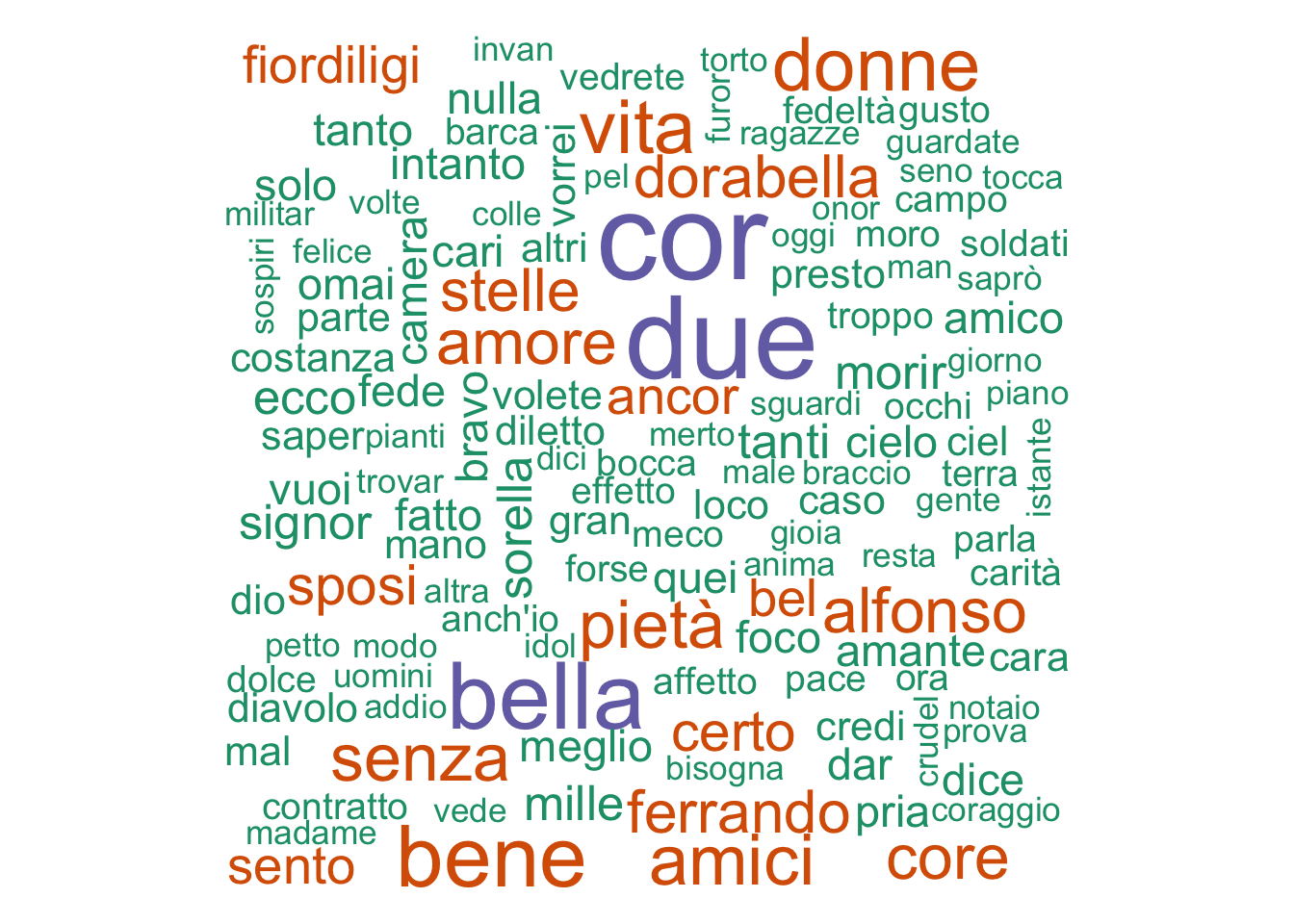
Unsurprisingly the main characters’ names are very common, but we also have “pieta” (pity); “amici” (friends); “amor” (love); “stelle” (stars). How do these compare to another Mozart and Da Ponte collaboration, Don Giovanni?
# Load in all of the different scenes
# If you are having encoding issues try the encoding argument
# dona1s1 <- readLines("giovanni/a1s1.txt", encoding = "UTF-8")
dona1s1 <- readLines("giovanni/a1s1.txt")
dona1s2 <- readLines("giovanni/a1s2.txt")
dona1s2 <- readLines("giovanni/a1s2.txt")
dona1s3 <- readLines("giovanni/a1s3.txt")
dona1s4 <- readLines("giovanni/a1s4.txt")
dona1s5 <- readLines("giovanni/a1s5.txt")
dona1s6 <- readLines("giovanni/a1s6.txt")
dona1s7 <- readLines("giovanni/a1s7.txt")
dona1s8 <- readLines("giovanni/a1s8.txt")
dona1s9 <- readLines("giovanni/a1s9.txt")
dona1s10 <- readLines("giovanni/a1s10.txt")
dona1s11 <- readLines("giovanni/a1s11.txt")
dona1s12 <- readLines("giovanni/a1s12.txt")
dona1s13 <- readLines("giovanni/a1s13.txt")
dona1s14 <- readLines("giovanni/a1s14.txt")
dona1s15 <- readLines("giovanni/a1s15.txt")
dona1s16 <- readLines("giovanni/a1s16.txt")
dona1s17 <- readLines("giovanni/a1s17.txt")
dona1s18 <- readLines("giovanni/a1s18.txt")
dona1s19 <- readLines("giovanni/a1s19.txt")
dona1s20 <- readLines("giovanni/a1s20.txt")
dona2s1 <- readLines("giovanni/a2s1.txt")
dona2s2 <- readLines("giovanni/a2s2.txt")
dona2s3 <- readLines("giovanni/a2s3.txt")
dona2s4 <- readLines("giovanni/a2s4.txt")
dona2s5 <- readLines("giovanni/a2s5.txt")
dona2s6 <- readLines("giovanni/a2s6.txt")
dona2s7 <- readLines("giovanni/a2s7.txt")
dona2s8 <- readLines("giovanni/a2s8.txt")
dona2s9 <- readLines("giovanni/a2s9.txt")
dona2s10 <- readLines("giovanni/a2s10.txt")
dona2s11 <- readLines("giovanni/a2s11.txt")
dona2s12 <- readLines("giovanni/a2s12.txt")
dona2s13 <- readLines("giovanni/a2s13.txt")
dona2s14 <- readLines("giovanni/a2s14.txt")
dona2s15 <- readLines("giovanni/a2s15.txt")
dona2s16 <- readLines("giovanni/a2s16.txt")


# Turn them all into  data frames so it's easier to work with
dona1s1 <- data_frame(text = dona1s1)
dona1s2 <- data_frame(text = dona1s2)
dona1s3 <- data_frame(text = dona1s3)
dona1s4 <- data_frame(text = dona1s4)
dona1s5 <- data_frame(text = dona1s5)
dona1s6 <- data_frame(text = dona1s6)
dona1s7 <- data_frame(text = dona1s7)
dona1s8 <- data_frame(text = dona1s8)
dona1s9 <- data_frame(text = dona1s9)
dona1s10 <- data_frame(text = dona1s10)
dona1s11 <- data_frame(text = dona1s11)
dona1s12 <- data_frame(text = dona1s12)
dona1s13 <- data_frame(text = dona1s13)
dona1s14 <- data_frame(text = dona1s14)
dona1s15 <- data_frame(text = dona1s15)
dona1s16 <- data_frame(text = dona1s16)
dona1s17 <- data_frame(text = dona1s17)
dona1s18 <- data_frame(text = dona1s18)
dona1s19 <- data_frame(text = dona1s19)
dona1s20 <- data_frame(text = dona1s20)
dona2s1 <- data_frame(text = dona2s1)
dona2s2 <- data_frame(text = dona2s2)
dona2s3 <- data_frame(text = dona2s3)
dona2s4 <- data_frame(text = dona2s4)
dona2s5 <- data_frame(text = dona2s5)
dona2s6 <- data_frame(text = dona2s6)
dona2s7 <- data_frame(text = dona2s7)
dona2s8 <- data_frame(text = dona2s8)
dona2s9 <- data_frame(text = dona2s9)
dona2s10 <- data_frame(text = dona2s10)
dona2s11 <- data_frame(text = dona2s11)
dona2s12 <- data_frame(text = dona2s12)
dona2s13 <- data_frame(text = dona2s13)
dona2s14 <- data_frame(text = dona2s14)
dona2s15 <- data_frame(text = dona2s15)
dona2s16 <- data_frame(text = dona2s16)
# Combine these data frames (help from https://www.r-bloggers.com/concatenating-a-list-of-data-frames/)
giovanniDF <- rbind.fill(dona1s1, dona1s2, dona1s3, dona1s4, dona1s5, dona1s6, dona1s7, dona1s8, dona1s9, dona1s10, dona1s11, dona1s12, dona1s13, dona1s14, dona1s15, dona1s16, dona2s1, dona2s2, dona2s3, dona2s4, dona2s5, dona2s6, dona2s7, dona2s8, dona2s9, dona2s10, dona2s11, dona2s12, dona2s13, dona2s14, dona2s15, dona2s16)
# NOTE TO SELF TRY DOING THESE BEFORE EVERYTHING ELSE
giovanniDF$text <- gsub("NO.","", giovanniDF$text)
giovanniDF$text <- gsub("RECITATIVO","", giovanniDF$text)
giovanniDF$text <- gsub("ACCOMPAGNATO","", giovanniDF$text)
giovanniDF$text <- gsub("ARIA","", giovanniDF$text)
giovanniDF$text <- gsub("DUETTO","", giovanniDF$text)
giovanniDF$text <- gsub("TERZETTO","", giovanniDF$text)
giovanniDF$text <- gsub("QUARTETTO","", giovanniDF$text)
giovanniDF$text <- gsub("QUINTETTO","", giovanniDF$text)
giovanniDF$text <- gsub("SESTETTO","", giovanniDF$text)
# Let's get rid of stage directions (help from https://stackoverflow.com/questions/13529360/replace-text-within-parenthesis-in-r)
giovanniDF$text <- gsub( " *\\(.*?\\) *", "", giovanniDF$text)
# Also get rid of numbers (help from here: http://www.endmemo.com/program/R/gsub.php)
giovanniDF$text <- gsub("\\d+","", giovanniDF$text)
# Get rid of "d'" a shortening of "di" (easier to do it this way than as a stop word)
giovanniDF$text <- gsub("d'","", giovanniDF$text)
# Get rid of "dell'", a shortening of "dello/a/gli/i"
giovanniDF$text <- gsub("dell'","", giovanniDF$text)
# Get rid of "l'" a shortening of "la" or "il" in front of words that start with a vowel
giovanniDF$text <- gsub("l'","", giovanniDF$text)
# There are some issues with this libretto, I have to make sure it can pick up the names as separate things
giovanniDF$text <- gsub("DONNA","", giovanniDF$text)
giovanniDF$text <- gsub("DON","", giovanniDF$text)
# Let's transform this into transcript form
# First label whether a row is a line or character name
# Create a data frame with the character names that exist in the text
doncharacters = c("GIOVANNI", "ANNA", "LEPORELLO", "COMMENDATORE", "OTTAVIO", "ELVIRA", "ZERLINA", "MASETTO", "COMMENDATORE", "CONTADINE", "CONTADINI", "CORO")
donchardf <- data.frame(doncharacters)
# Now use regular expression to identify when the row is a character name (TRUE) or not (FALSE)
# FALSE then means that we are looking at a line row
donchargrepl <- grepl(paste(donchardf$doncharacters, collapse = "|"), giovanniDF$text)
# This says go through each row and if something in that row is the same as something in our characters data frame (the "|" is working as an 'or', telling R that it could be Dorabella or Fiordiligi or Don Alfonso, etc.) then put 'TRUE'
# The output is a list so we have to turn it into a data frame to merge it back with our data
donchargreplDF <-as.data.frame(donchargrepl)
# To merge something, you have to have a common key. Create an id row for each data frame you want to combine and that will be your key!
giovanniDF$id <- 1:nrow(giovanniDF)
donchargreplDF$id <- 1:nrow(donchargreplDF)
# Now merge!
dontext_df <- merge(giovanniDF,donchargreplDF,by="id")
# Now things get complicated. We are going to 'group' things according to names. We have name rows represented by 'TRUE' and lines represented by 'FALSE'. So we can create a group by telling R to make a new id row that starts anew each time it sees 'TRUE'.
# Make groups of lines associated with names (help from here https://stackoverflow.com/questions/29376178/count-changes-to-contents-of-a-character-vector)
dontest_df <- dontext_df %>% mutate(
try_1 = cumsum(ifelse(donchargrepl == TRUE, 1, 0))
)
# Now we want to copy our text column so we can eventually have two columns in which one has all of the lines and the other has the characters speaking those lines
# Create a duplicate column of the text
dontest_df$text2 <- dontest_df$text
# Let's get rid of superfluous info for our character column (so, in this case, lines)
# Get rid of lines in one column
dontest_df$text <- ifelse(dontest_df$donchargrepl == TRUE, dontest_df$text, "")
# This command says look through the text column and if the corresponding chargrepl column (our logical vector) is TRUE leave it alone but if it is else ('ifelse') replace with "" (nothing).
# Do the same for the other text column, but opposite
dontest_df$text2 <- ifelse(dontest_df$donchargrepl == FALSE, dontest_df$text2, "")
# Now let's aggregate things
donresult <- aggregate(text ~ try_1, data = dontest_df, paste, collapse = "")
donresult2 <- aggregate(text2 ~ try_1, data = dontest_df, paste, collapse = "")
# These commands are creating two data frames. The first one is just character names, the second is the lines associated with those characters. The collapse is also helping us out in that it's putting each series of phrases in one cell. That's because we are collapsing by the group id we created a few steps back ('try_1').
# Now we merge these data frames together by their shared column of group id
new_giovanni <- merge(donresult, donresult2, by="try_1")
# Let's get rid of that id!
new_giovanni <- new_giovanni[,c("text","text2")]# Transform this into something we can work with: tidy text!
tidy_giovanni <- new_giovanni %>%
unnest_tokens(word, text2)
# Get rid of stop words
giovannitribble <- tidy_giovanni %>%
anti_join(itstopwords)
giovannifreq <- giovannitribble %>%
count(word, sort = TRUE) wordcloud(giovannifreq$word,giovannifreq$n, min.freq=5,
colors=brewer.pal(1, "Dark2"))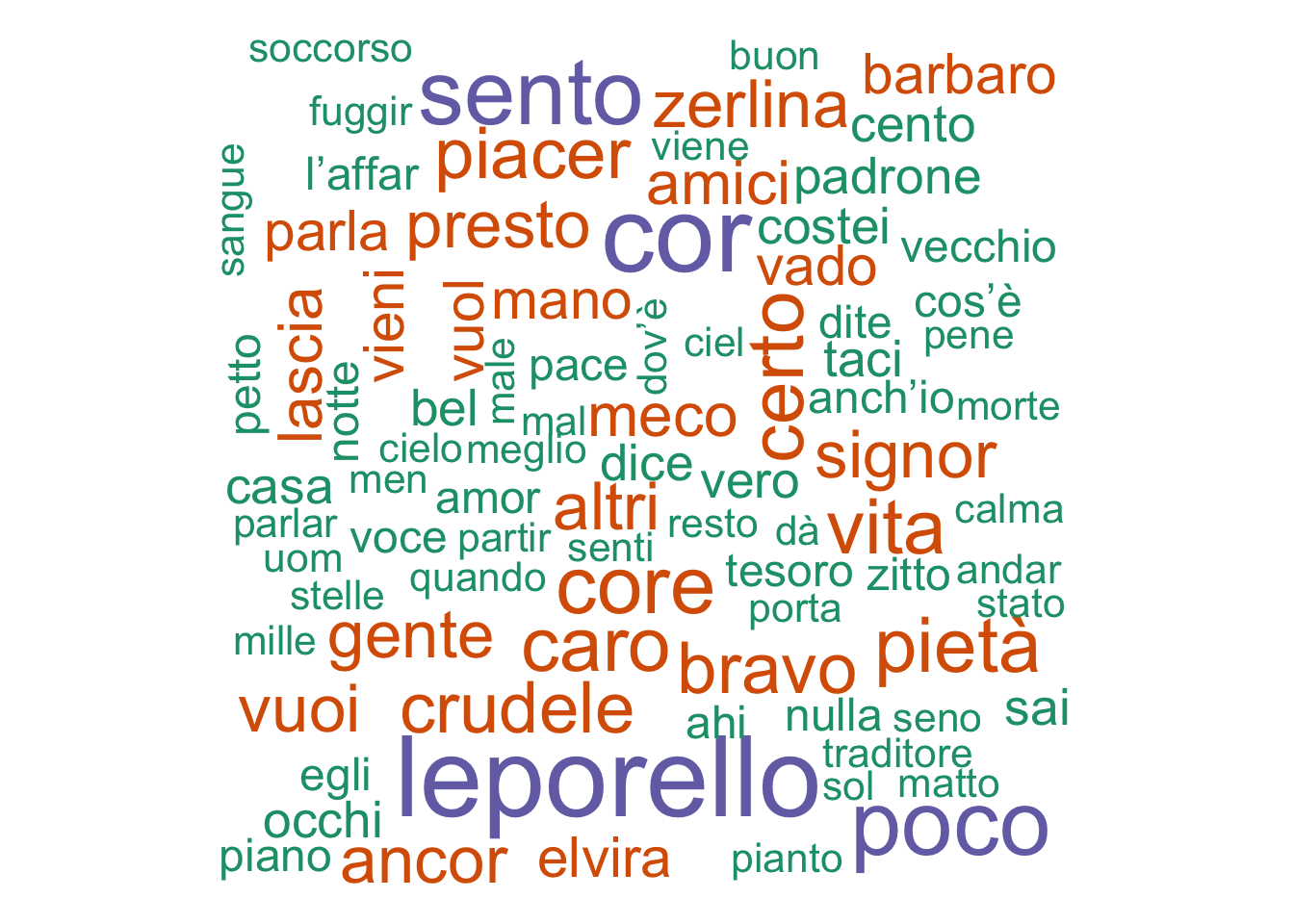
We do see some differences even here – Cosi has mention of friends, heart, love, etc. while Giovanni has some more negative words like “barbaro”. Both clearly are tied to the individual plots of the operas (you can tell which word cloud belongs where!)
To round it out let’s do the last famous Da Ponte - Mozart colab, Le Nozze Di Figaro. This one is all in one document, so it’ll require less work to load it in.
figaro <- readLines("figaro/figaro.txt")

figaroDF <- data_frame(text = figaro)

# Let's get rid of stage directions (help from https://stackoverflow.com/questions/13529360/replace-text-within-parenthesis-in-r)
figaroDF$text <- gsub( " *\\(.*?\\) *", "", figaroDF$text)

# Get rid of everything between '< >' -- this is how arias and recits have been marked in this libretto
figaroDF$text <- gsub("<[^>]+>", "", figaroDF$text)

# There are also some instances in which quotations are used, let's get rid of those too
figaroDF$text <- gsub( '"', '', figaroDF$text)
# Note we chanage " to ' in the gsub function to not confuse R -- if we had """ R wouldn't know what to do with that because it would read it as one quotation ending and another incomplete one.

# Also get rid of numbers (help from here: http://www.endmemo.com/program/R/gsub.php)
figaroDF$text <- gsub("\\d+","", figaroDF$text)
# Get rid of "d'" a shortening of "di" (easier to do it this way than as a stop word)
figaroDF$text <- gsub("d'","", figaroDF$text)
# Get rid of "dell'", a shortening of "dello/a/gli/i"
figaroDF$text <- gsub("dell'","", figaroDF$text)
# You have to do this before l' because R would get rid of the "l'" of "dell'", leaving you with "del" smooshed onto the next word, which is not what you want!
# Get rid of "l'" a shortening of "la" or "il" in front of words that start with a vowel
figaroDF$text <- gsub("l'","", figaroDF$text)

# There are some issues with this libretto, I have to make sure it can pick up the names as separate things
# figaroDF$text <- gsub("DONNA","", figaroDF$text)
# figaroDF$text <- gsub("DON","", figaroDF$text)

# Let's transform this into transcript form
# First label whether a row is a line or character name

# Create a data frame with the character names that exist in the text
figcharacters = c("IL CONTE", "LA CONTESSA", "SUSANNA", "FIGARO", "CHERUBINO", "MARCELLINA", "BARTOLO",  "BASILIO", "DON CURZIO", "BARBARINA", "ANTONIO", "DUE DONNE", "TUTTI", "CORO", "CONTADINELLE")
figchardf <- data.frame(figcharacters)

# Now use regular expression to identify when the row is a character name (TRUE) or not (FALSE)
# FALSE then means that we are looking at a line row
figchargrepl <- grepl(paste(figchardf$figcharacters, collapse = "|"), figaroDF$text)
# This says go through each row and if something in that row is the same as something in our characters data frame (the "|" is working as an 'or', telling R that it could be Dorabella or Fiordiligi or Don Alfonso, etc.) then put 'TRUE'

# The output is a list so we have to turn it into a data frame to merge it back with our data
figchargreplDF <-as.data.frame(figchargrepl)

# To merge something, you have to have a common key. Create an id row for each data frame you want to combine and that will be your key!
figaroDF$id <- 1:nrow(figaroDF)
figchargreplDF$id <- 1:nrow(figchargreplDF)

# Now merge!
figtext_df <- merge(figaroDF,figchargreplDF,by="id")

# Now things get complicated. We are going to 'group' things according to names. We have name rows represented by 'TRUE' and lines represented by 'FALSE'. So we can create a group by telling R to make a new id row that starts anew each time it sees 'TRUE'.

# Make groups of lines associated with names (help from here https://stackoverflow.com/questions/29376178/count-changes-to-contents-of-a-character-vector)
figtest_df <- figtext_df %>% mutate(
   try_1 = cumsum(ifelse(figchargrepl == TRUE, 1, 0))
   )

# Now we want to copy our text column so we can eventually have two columns in which one has all of the lines and the other has the characters speaking those lines
# Create a duplicate column of the text
figtest_df$text2 <- figtest_df$text

# Let's get rid of superfluous info for our character column (so, in this case, lines)
# Get rid of lines in one column
figtest_df$text <- ifelse(figtest_df$figchargrepl == TRUE, figtest_df$text, "")
# This command says look through the text column and if the corresponding chargrepl column (our logical vector) is TRUE leave it alone but if it is else ('ifelse') replace with "" (nothing).

# Do the same for the other text column, but opposite
figtest_df$text2 <- ifelse(figtest_df$figchargrepl == FALSE, figtest_df$text2, "")

# Now let's aggregate things
figresult <- aggregate(text ~ try_1, data = figtest_df, paste, collapse = "")
figresult2 <- aggregate(text2 ~ try_1, data = figtest_df, paste, collapse = "")
# These commands are creating two data frames. The first one is just character names, the second is the lines associated with those characters. The collapse is also helping us out in that it's putting each series of phrases in one cell. That's because we are collapsing by the group id we created a few steps back ('try_1').

# Now we merge these data frames together by their shared column of group id
new_figaro <- merge(figresult, figresult2, by="try_1")

# Let's get rid of that id!
new_figaro <- new_figaro[,c("text","text2")]
# Transform this into something we can work with: tidy text!
tidy_figaro <- new_figaro %>%
unnest_tokens(word, text2)
figtribble <- tidy_figaro %>%
anti_join(itstopwords)
figfreq <- figtribble %>%
count(word, sort = TRUE) wordcloud(figfreq$word,figfreq$n, min.freq=7,
colors=brewer.pal(1, "Dark2"))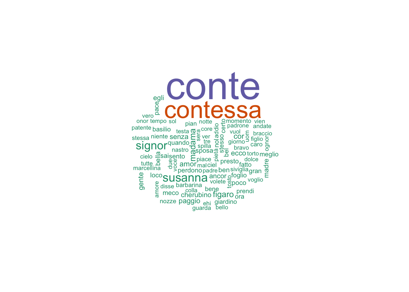
Let’s look at some bigrams / trigrams
fig_bigrams <- new_figaro %>%
  unnest_tokens(bigram, text2, token = "ngrams", n = 2)

figbigrams_separated <- fig_bigrams %>%
  separate(bigram, c("word1", "word2"), sep = " ")

figbigrams_filtered <- figbigrams_separated %>%
  filter(!word1 %in% itstopwords$word) %>%
  filter(!word2 %in% itstopwords$word)

# new bigram counts:
figbigram_counts <- figbigrams_filtered %>%
  count(word1, word2, sort = TRUE)

figbigram_counts
## # A tibble: 1,763 x 3
## word1 word2 n
## <chr> <chr> <int>
## 1 signor conte 6
## 2 conte susanna 5
## 3 conte olà 4
## 4 saggio signor 4
## 5 ballare signor 3
## 6 conte ebben 3
## 7 olà silenzio 3
## 8 pace pace 3
## 9 parlo amor 3
## 10 perdono perdono 3
## # ... with 1,753 more rowsInterestingly for an opera (which might suggest certain phrases being repeated multiple times) we have few bigrams. We see some repeats for the chorus “Bella Vita Militar”, for example.
What about trigrams?
new_figaro %>%
  unnest_tokens(trigram, text2, token = "ngrams", n = 3) %>%
  separate(trigram, c("word1", "word2", "word3"), sep = " ") %>%
  filter(!word1 %in% itstopwords$word,
         !word2 %in% itstopwords$word,
         !word3 %in% itstopwords$word) %>%
  count(word1, word2, word3, sort = TRUE)
## # A tibble: 708 x 4
## word1 word2 word3 n
## <chr> <chr> <chr> <int>
## 1 ballare signor contino 3
## 2 conte olà silenzio 3
## 3 vuol ballare signor 3
## 4 amanti costanti seguaci 2
## 5 amor donne vedete 2
## 6 bel fiore almo 2
## 7 bel guadagno colla 2
## 8 conte gente gente 2
## 9 costanti seguaci onor 2
## 10 donne vedete s'io 2
## # ... with 698 more rowsAgain, trigrams aren’t THAT helpful when looking at things like an opera, because part of the structure of opera (at least at this time) was to have a specific structure to arias, in which certain phrases would be repeated. This might be more insightful if you want to look at bigrams in a varied, larger data set, like a bunch of tweets or maybe a corpus of newspaper data. Or we could combine all of our operas and look at bigrams to see if there are any instances of two words happening together. First though, let’s compare at how ‘love’ is discussed in each of these operas.
figbigrams_filtered %>%
  filter(word1 == "amore") %>%
  count(word2, sort = TRUE)
## # A tibble: 3 x 2
## word2 n
## <chr> <int>
## 1 ch'oggi 1
## 2 l'abito 1
## 3 unita 1# Sometimes this is shortened
figbigrams_filtered %>%
filter(word1 == "amor") %>%
count(word2, sort = TRUE)## # A tibble: 4 x 2
## word2 n
## <chr> <int>
## 1 donne 2
## 2 pace 1
## 3 sognando 1
## 4 vegliando 1# Sometimes 'amore' is the second word, not the first (flexible word order here)
figbigrams_filtered %>%
filter(word2 == "amore") %>%
count(word1, sort = TRUE)## # A tibble: 6 x 2
## word1 n
## <chr> <int>
## 1 cherubin 1
## 2 man 1
## 3 mentono 1
## 4 ove 1
## 5 sforza 1
## 6 spagna 1figbigrams_filtered %>%
filter(word2 == "amor") %>%
count(word1, sort = TRUE)## # A tibble: 10 x 2
## word1 n
## <chr> <int>
## 1 parlo 3
## 2 adoncino 1
## 3 antico 1
## 4 felice 1
## 5 intendete 1
## 6 nomi 1
## 7 piaceri 1
## 8 porgi 1
## 9 solo 1
## 10 tenero 1See how it takes a few tries to get something that makes more sense with the data? In this instance, we see that looking at where the shortened ‘amor’ pops up as the second word gives us a little more information about how love is discussed in Le Nozze di Figaro.
Let’s look at Don Giovanni now…
don_bigrams <- new_giovanni %>%
  unnest_tokens(bigram, text2, token = "ngrams", n = 2)

donbigrams_separated <- don_bigrams %>%
  separate(bigram, c("word1", "word2"), sep = " ")

donbigrams_filtered <- donbigrams_separated %>%
  filter(!word1 %in% itstopwords$word) %>%
  filter(!word2 %in% itstopwords$word)

# Let's check out 'love'!

# donbigrams_filtered %>%
#   filter(word1 == "amore") %>%
#   count(word2, sort = TRUE)
# No instances for this one

# Sometimes this is shortened

donbigrams_filtered %>%
  filter(word1 == "amor") %>%
  count(word2, sort = TRUE)
## # A tibble: 1 x 2
## word2 n
## <chr> <int>
## 1 consiglio 1# Sometimes 'amore' is the second word, not the first (flexible word order here)
donbigrams_filtered %>%
filter(word2 == "amore") %>%
count(word1, sort = TRUE)## # A tibble: 2 x 2
## word1 n
## <chr> <int>
## 1 fingere 1
## 2 parla 1donbigrams_filtered %>%
filter(word2 == "amor") %>%
count(word1, sort = TRUE)## # A tibble: 4 x 2
## word1 n
## <chr> <int>
## 1 fido 2
## 2 innocente 1
## 3 sorte 1
## 4 tenero 1Again we see the last one is more effective in picking up examples. Already we can see a shift in tone from Figaro to Giovanni – “fingere” for example means to pretend or fake.
How about Cosi?
bigrams_filtered %>%
  filter(word1 == "amore") %>%
  count(word2, sort = TRUE)
## # A tibble: 6 x 2
## word2 n
## <chr> <int>
## 1 altri 1
## 2 d'esca 1
## 3 en 1
## 4 esempi 1
## 5 singolar 1
## 6 terminar 1# Sometimes this is shortened
bigrams_filtered %>%
filter(word1 == "amor") %>%
count(word2, sort = TRUE)## # A tibble: 7 x 2
## word2 n
## <chr> <int>
## 1 andate 1
## 2 contentissimi 1
## 3 lega 1
## 4 secondate 1
## 5 simile 1
## 6 virtuoso 1
## 7 vista 1# Sometimes 'amore' is the second word, not the first (flexible word order here)
bigrams_filtered %>%
filter(word2 == "amore") %>%
count(word1, sort = TRUE)## # A tibble: 7 x 2
## word1 n
## <chr> <int>
## 1 balsamo 1
## 2 cangiano 1
## 3 desio 1
## 4 giusto 1
## 5 intatto 1
## 6 speme 1
## 7 trattar 1bigrams_filtered %>%
filter(word2 == "amor") %>%
count(word1, sort = TRUE)## # A tibble: 11 x 2
## word1 n
## <chr> <int>
## 1 alfonso 1
## 2 antidoto 1
## 3 dio 1
## 4 madame 1
## 5 mangia 1
## 6 pennacchi 1
## 7 senza 1
## 8 sola 1
## 9 tenero 1
## 10 vezzosi 1
## 11 voci 1Let’s combine all of these data frames together to look at everything at once. Let’s build a mini Mozart opera corpus.
# Let's first add columns so we know which line belongs to which opera
# Let's also add an 'id' -- this will be helpful later when we want to look at sentiment changes over time
new_data$opera <- "COSI"
new_data$id <- 1:nrow(new_data)
new_giovanni$opera<-"GIOVANNI"
new_giovanni$id <- 1:nrow(new_giovanni)
new_figaro$opera<-"FIGARO"
new_figaro$id <- 1:nrow(new_figaro)

mozart <- rbind.fill(new_data, new_giovanni, new_figaro)

#Let's play around with this and look at a word cloud representation
tidy_mozart <- mozart %>%
  unnest_tokens(word, text2)

moztribble <- tidy_mozart %>%
  anti_join(itstopwords)

mozartfreq <- moztribble %>%
  count(word, sort = TRUE)

# Because we have more words, let's up the minimum frequency to 10
wordcloud(mozartfreq$word,mozartfreq$n, min.freq=10,
          colors=brewer.pal(1, "Dark2"))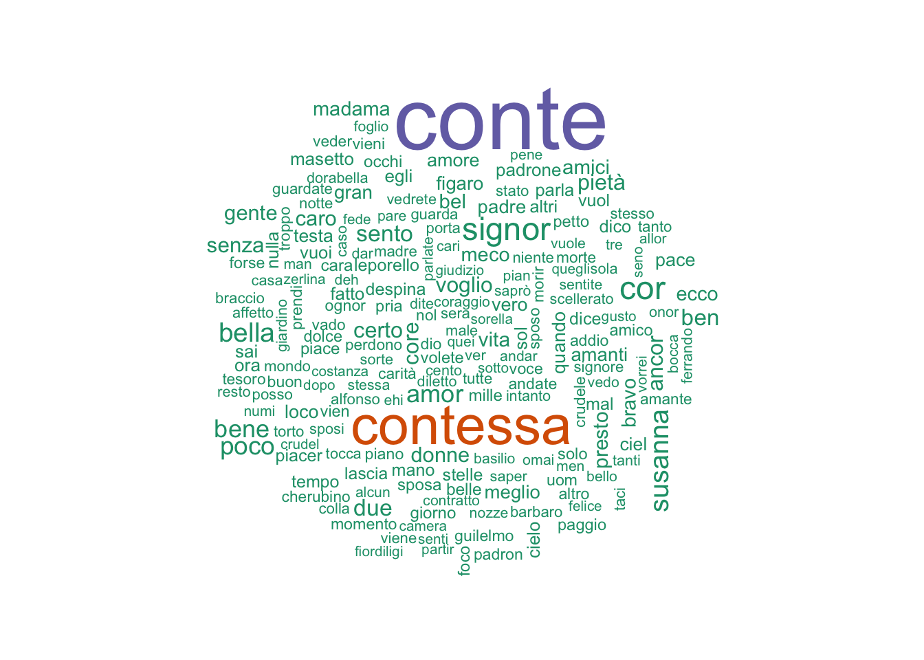
We don’t have the best sentiment dictionary for Italian (especially this kind of Italian, which is 200+ years old!) nor do we have a ‘built in’ sentiment dictionary from a package. If we were working with English, we could use the tidytext package to download the Bing sentiment corpus and use that, etc. But we will have to make our own! I’ll be using the sentiment dictionary Andrea Cirillo put together to look at Italian tweets, available here.
# First let's load in some text files, which are just the words Andrea has collected that I copy-pasted into a word doc and 'saved as' a txt file.
pos <- readLines("itpositivewords.txt")
neg <- readLines("itnegativewords.txt")

# Turn these into data frames
posDF <- data_frame(text = pos)
negDF <- data_frame(text = neg)

# Create a new column for each with a marker of what kind of sentiment we are dealing with
posDF$sentiment <- "positive"
negDF$sentiment <- "negative"

# Combine these into a data frame
sentiment <- rbind.fill(posDF, negDF)

# We have lots of empty cells, get rid of those
# Mark empty cells as NA
sentiment$text[sentiment$text==""] <- NA

# Get rid of NA rows (help from here: https://stackoverflow.com/questions/12763890/exclude-blank-and-na-in-r)
sentimentDF <- na.omit(sentiment)
Now that we have our own new sentiment dictionary, let’s evaluate the sentiment of our operas! Code adapted from Silge and Robinson.
# We have to change the name again
names(sentimentDF)[names(sentimentDF)=="text"] <- "word"

## Sentiment analysis
senti_word_counts <- tidy_mozart %>%
  inner_join(sentimentDF) %>%
  count(word, sentiment, sort = TRUE) %>%
  ungroup()

# senti_word_counts

# The first time I ran this, I didn't get too many matches. Then I went back to the text file, added some words to both postive and negative text files and now we have a semblance of a result. Hopefully you'll have more luck with your more contemporary texts!

# Now we can graph these
senti_word_counts %>%
  filter(n > 15) %>%
  mutate(n = ifelse(sentiment == "negative", -n, n)) %>%
  mutate(word = reorder(word, n)) %>%
  ggplot(aes(word, n, fill = sentiment)) +
  geom_bar(alpha = 0.8, stat = "identity") +
  labs(y = "Contribution to sentiment",
       x = NULL) +
  coord_flip()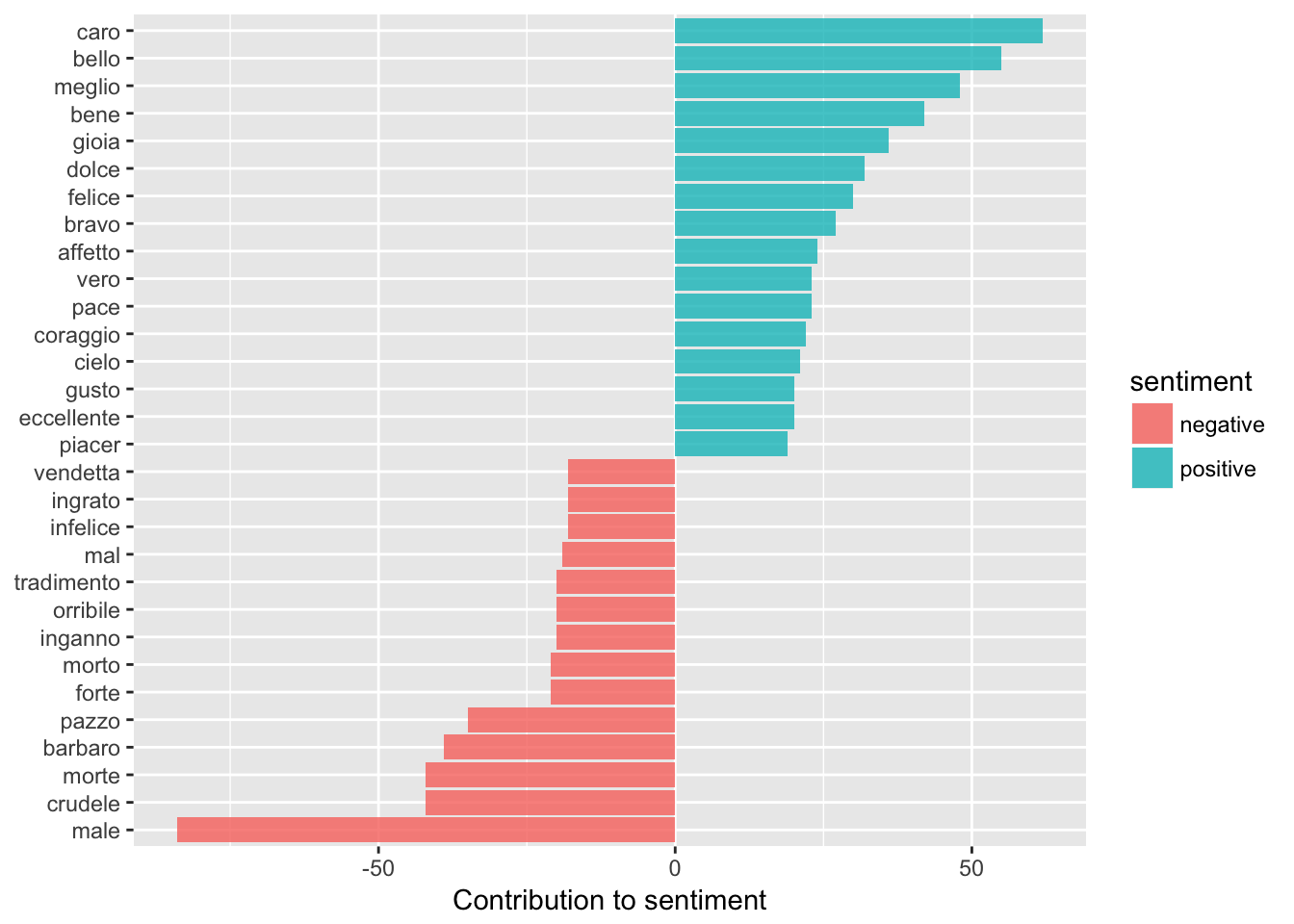
You will most likely have to fiddle with this a bit, depending on your data and ESPECIALLY if you’ve ‘made’ your own sentiment dictionary. For example, the first time I ran this, it was counting ‘caro’ as both positive and negative. This is because ‘caro’ means ‘dear’ – which in operas is usually used as a term of endearment, whereas in modern Italian it means expensive! So I had to go back to the negative sentiment list and delete it.
# Let's see how each opera compares
# Cosi
cosisenti_word_counts <- tribble %>%
  inner_join(sentimentDF) %>%
  count(word, sentiment, sort = TRUE) %>%
  ungroup()

cosisenti_word_counts %>%
  filter(n > 5) %>%
  mutate(n = ifelse(sentiment == "negative", -n, n)) %>%
  mutate(word = reorder(word, n)) %>%
  ggplot(aes(word, n, fill = sentiment)) +
  geom_bar(alpha = 0.8, stat = "identity") +
  labs(y = "Contribution to sentiment",
       x = NULL) +
  coord_flip()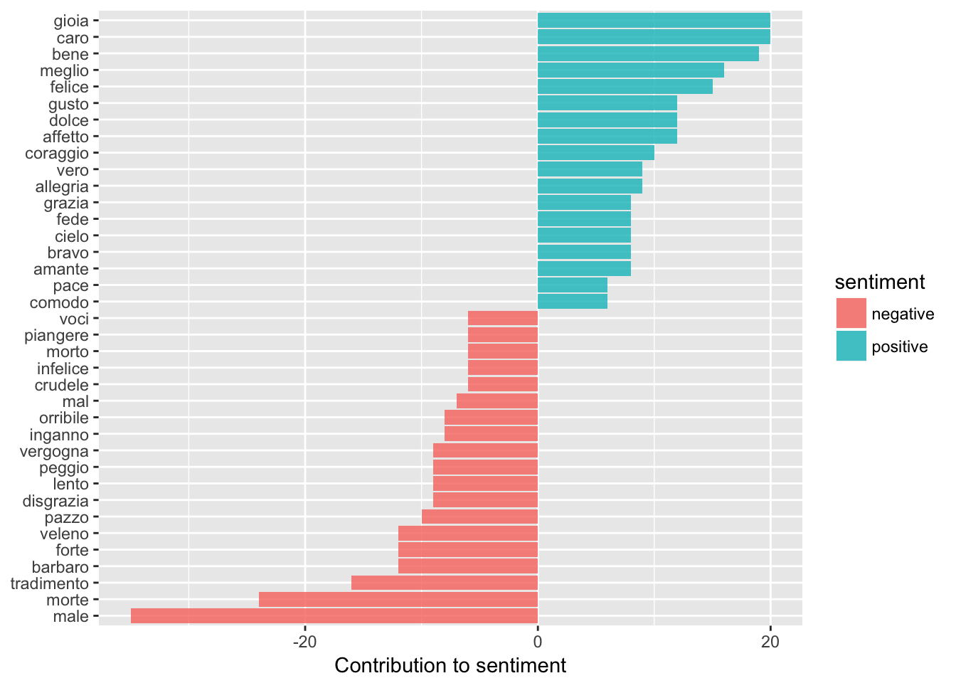
# Giovanni
donsenti_word_counts <- tidy_giovanni %>%
  inner_join(sentimentDF) %>%
  count(word, sentiment, sort = TRUE) %>%
  ungroup()

donsenti_word_counts %>%
  filter(n > 5) %>%
  mutate(n = ifelse(sentiment == "negative", -n, n)) %>%
  mutate(word = reorder(word, n)) %>%
  ggplot(aes(word, n, fill = sentiment)) +
  geom_bar(alpha = 0.8, stat = "identity") +
  labs(y = "Contribution to sentiment",
       x = NULL) +
  coord_flip()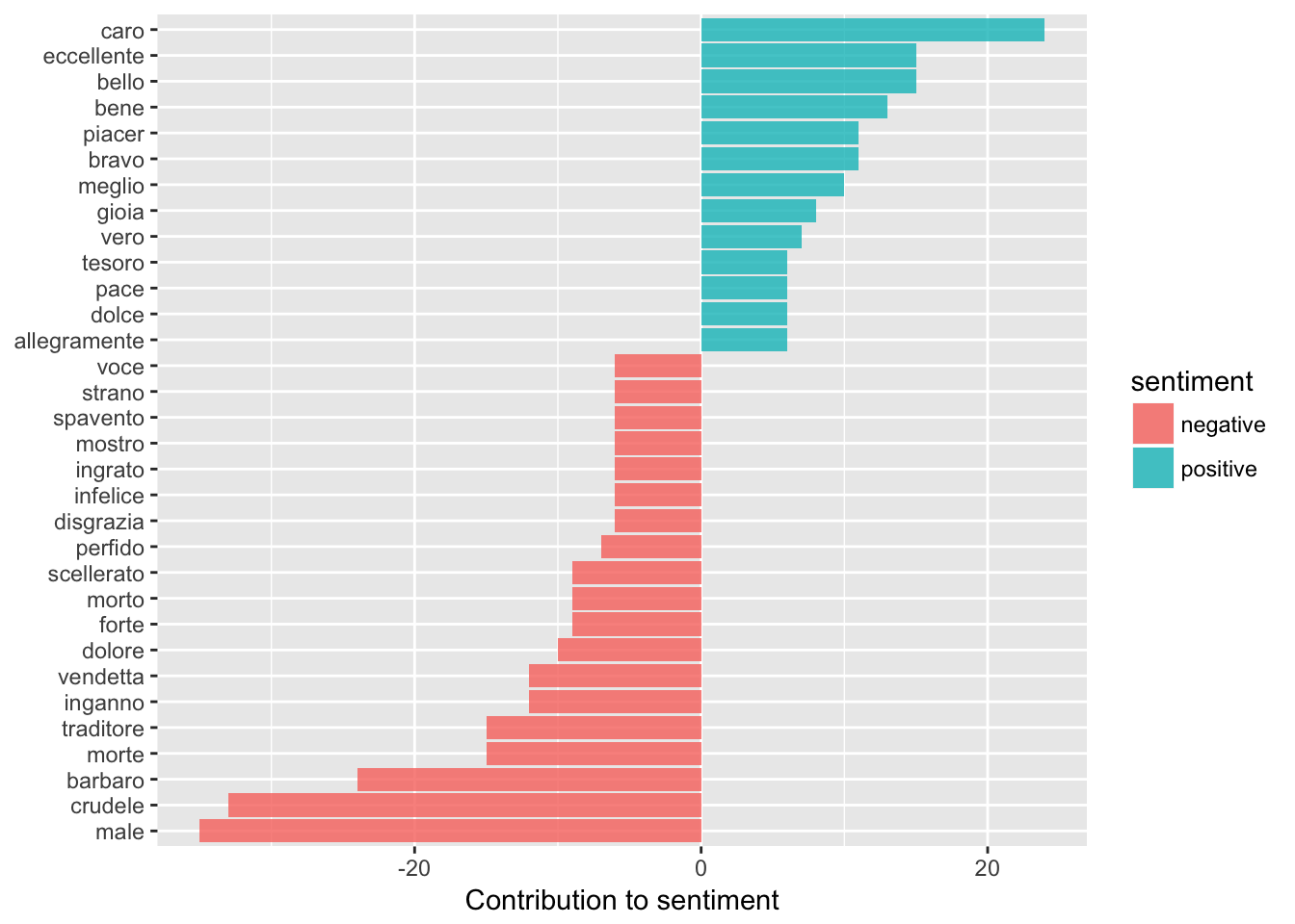
# Figaro
figsenti_word_counts <- tidy_figaro %>%
  inner_join(sentimentDF) %>%
  count(word, sentiment, sort = TRUE) %>%
  ungroup()

figsenti_word_counts %>%
  filter(n > 5) %>%
  mutate(n = ifelse(sentiment == "negative", -n, n)) %>%
  mutate(word = reorder(word, n)) %>%
  ggplot(aes(word, n, fill = sentiment)) +
  geom_bar(alpha = 0.8, stat = "identity") +
  labs(y = "Contribution to sentiment",
       x = NULL) +
  coord_flip()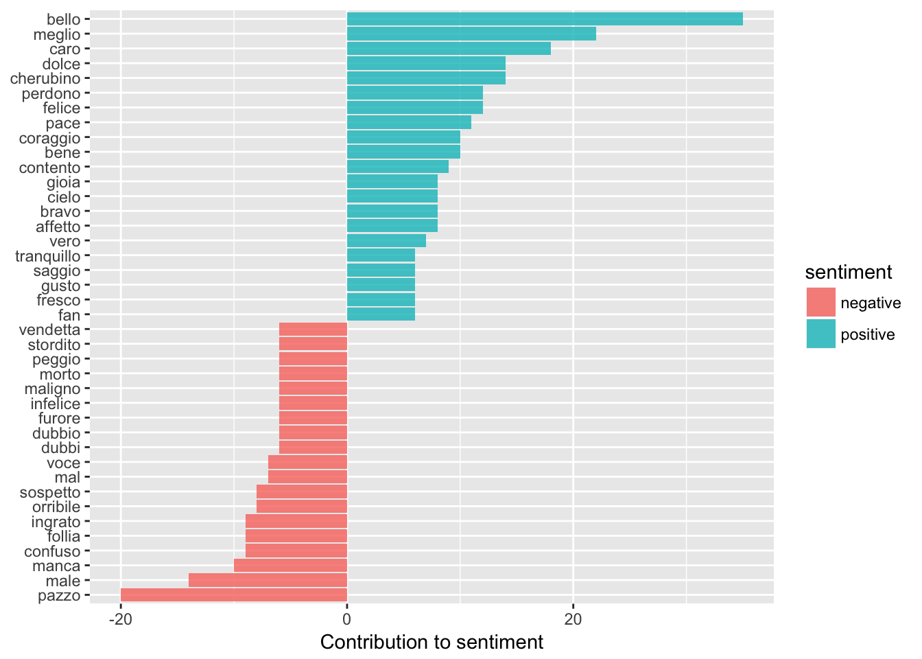
As we might guess, the opera seria (‘serious’ or melodramatic opera) Don Giovanni seems to be skewed on the negative side, however the two opera buffas (comedic operas) do not follow this pattern. Cosi Fan Tutte has a lot of negative sentiment, more than positive sentiment especially compared to Le Nozze di Figaro. This makes sense when we consider the plots (a lot of the opera is made up of pining; confusion and farewells) but it’s kind of interesting to see it scaled back a bit especially when we think about the tone of an opera overall and how words fit into that.
Something really cool to do would be to take advantage of opera as music drama by noting which key each of these words are being sung in (i.e. whether or not we are working in a major or minor key) to add an extra layer to our analysis, but that is a little too much work for the time being! This would be especially cool to try with Wagner, but I digress.
Let’s look at how sentiment has changed over the course of each opera! (Again, adapted from Silge and Robinson)
mozartsenti <- moztribble %>%
  inner_join(sentimentDF) %>%
  count(opera, index = id %/% 1, sentiment) %>%
  spread(sentiment, n, fill = 0) %>%
  mutate(sentiment = positive - negative)

# Graph
ggplot(mozartsenti, aes(index, sentiment, fill = opera)) +
  geom_col(show.legend = FALSE) +
  facet_wrap(~opera, ncol = 2, scales = "free_x")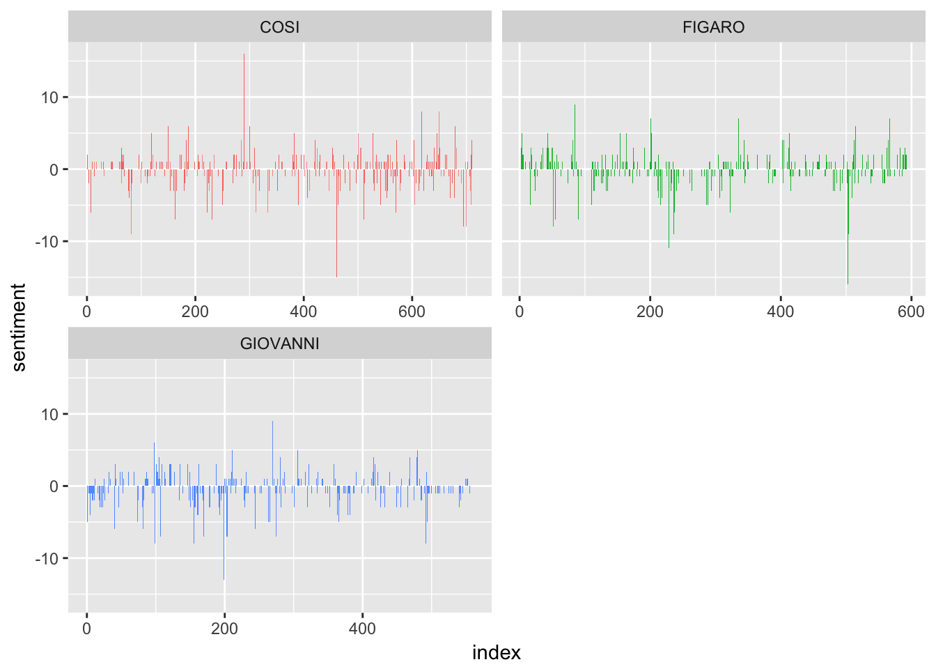
# That previous example was looking at line by line, but we can group these together a little more to see larger trends (you can modify this depending on your data)
mozartsenti <- moztribble %>%
  inner_join(sentimentDF) %>%
  count(opera, index = id %/% 10, sentiment) %>%
  spread(sentiment, n, fill = 0) %>%
  mutate(sentiment = positive - negative)

# Graph
ggplot(mozartsenti, aes(index, sentiment, fill = opera)) +
  geom_col(show.legend = FALSE) +
  facet_wrap(~opera, ncol = 2, scales = "free_x")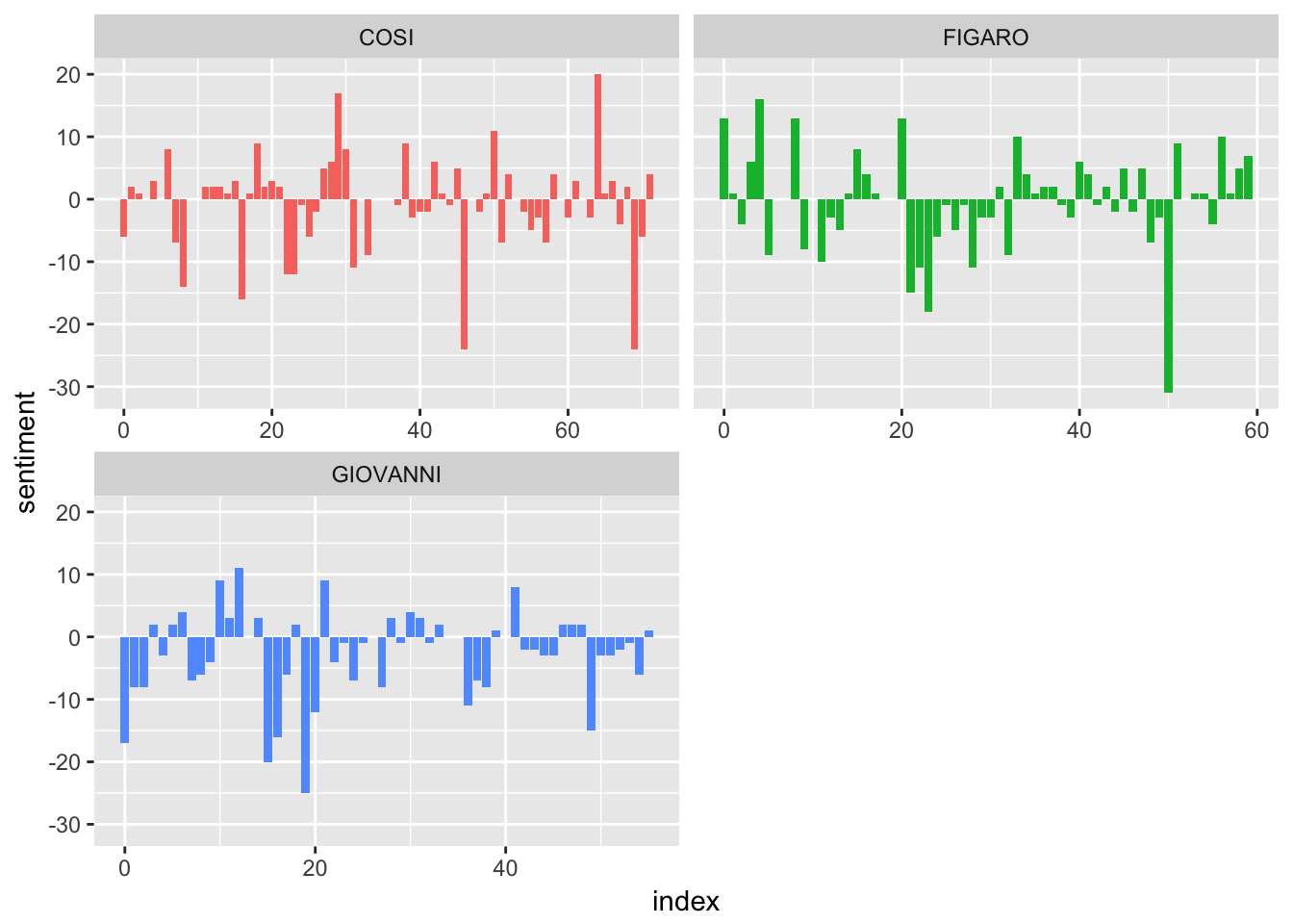
Let’s check out some more things. The following examples and code comes from Silge and Robinson’s Text Mining with R book which I have adapted for our data set that we’ve been working with.
Julia Silge’s blog also has a lot of cool examples of how to play around with these tools and how to get different visualizations.
# Use representation of text that has stop words removed
mozart_words <- moztribble %>%
  count(opera, word, sort = TRUE) %>%
  ungroup()

total_words <- mozart_words %>%
  group_by(opera) %>%
  summarize(total = sum(n))

mozart_words <- left_join(mozart_words, total_words)

mozart_words
## # A tibble: 6,441 x 4
## opera word n total
## <chr> <chr> <int> <int>
## 1 FIGARO conte 233 4838
## 2 FIGARO contessa 134 4838
## 3 FIGARO susanna 49 4838
## 4 FIGARO signor 46 4838
## 5 COSI cor 29 4200
## 6 COSI due 27 4200
## 7 FIGARO madama 25 4838
## 8 FIGARO figaro 24 4838
## 9 COSI amanti 22 4200
## 10 COSI bella 21 4200
## # ... with 6,431 more rowsAs Silge and Robinson explain (adapted to fit our example), now we have “one row in this mozart_words data frame for each word-opera combination; n is the number of times that word is used in that opera and total is the total words in that opera. The usual suspects are here with the highest n, “the”, “and”, “to”, and so forth (‘il’, ‘la’, ‘che’, etc.) … let’s look at the distribution of n/total for each opera, the number of times a word appears in an opera divided by the total number of terms (words) in that opera. This is exactly what term frequency is.”
Term frequency is an important concept in text mining. Let’s see some examples and explore what this term means and why it is useful.
ggplot(mozart_words, aes(n/total, fill = opera)) +
  geom_histogram(show.legend = FALSE) +
  xlim(NA, 0.0009) +
  facet_wrap(~opera, ncol = 2, scales = "free_y")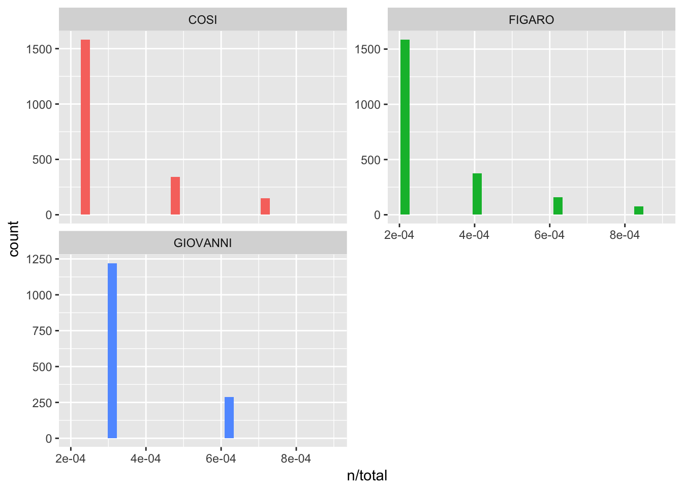
What this is trying to show is that “there are many words that occur rarely and fewer words that occur frequently”, a tenant of Zipf’s Law. Zipf’s Law is probably something you’ve heard of if you have taken corpus linguistics – it means “the frequency that a word appears is inversely proportionally to its rank”. We can see this with our own data (all code take from Silge and Robinson):
freq_by_rank <- mozart_words %>%
  group_by(opera) %>%
  mutate(rank = row_number(),
         `term frequency` = n/total)

# Better to plot to see relationship
freq_by_rank %>%
  ggplot(aes(rank, `term frequency`, color = opera)) +
  geom_line(size = 1.2, alpha = 0.8) +
  scale_x_log10() +
  scale_y_log10()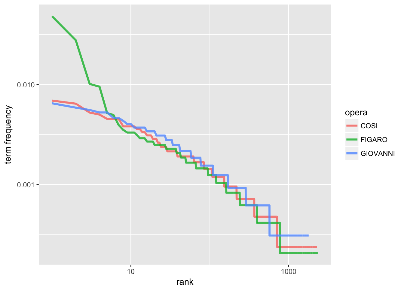
Kind of cool right? Anyway, the main idea that is useful for us out of this is thinking about the term-frequency / inverse document frequency representation of our data. As Silge and Robinson explain, “the idea of tf-idf is to find the important words for the content of each document by decreasing the weight for commonly used words and increasing the weight for words that are not used very much in a collection or corpus of documents” – basically, that if a word like ‘amor’ is really common across all of our librettos, it’s not really informative as to the unique character of each opera. If we are using text mining and analysis as a way to evaluate trends in our data, the tf-idf is really useful. It’s a way of seeing what are unique features in groupings of data. For example, if you have a collection of interviews on the same topic, what are some different features that come up for each person / interview session? If you are looking at a corpus of tweets collected by hashtag and have grouped them by time frame (let’s say grouped in terms of weeks) what are some unique terms for each time period? etc. etc.
# Let's get this td-idf started
mozart_words2 <- mozart_words %>%
  bind_tf_idf(word, opera, n)
mozart_words2
## # A tibble: 6,441 x 7
## opera word n total tf idf tf_idf
## <chr> <chr> <int> <int> <dbl> <dbl> <dbl>
## 1 FIGARO conte 233 4838 0.048160397 1.0986123 0.052909604
## 2 FIGARO contessa 134 4838 0.027697396 1.0986123 0.030428699
## 3 FIGARO susanna 49 4838 0.010128152 1.0986123 0.011126912
## 4 FIGARO signor 46 4838 0.009508061 0.0000000 0.000000000
## 5 COSI cor 29 4200 0.006904762 0.0000000 0.000000000
## 6 COSI due 27 4200 0.006428571 0.0000000 0.000000000
## 7 FIGARO madama 25 4838 0.005167425 0.0000000 0.000000000
## 8 FIGARO figaro 24 4838 0.004960728 1.0986123 0.005449916
## 9 COSI amanti 22 4200 0.005238095 0.4054651 0.002123865
## 10 COSI bella 21 4200 0.005000000 0.0000000 0.000000000
## # ... with 6,431 more rows# Look at high tf idf (i.e. terms that are most particular to certain operas)
mozart_words2 %>%
select(-total) %>%
arrange(desc(tf_idf))## # A tibble: 6,441 x 6
## opera word n tf idf tf_idf
## <chr> <chr> <int> <dbl> <dbl> <dbl>
## 1 FIGARO conte 233 0.048160397 1.098612 0.052909604
## 2 FIGARO contessa 134 0.027697396 1.098612 0.030428699
## 3 FIGARO susanna 49 0.010128152 1.098612 0.011126912
## 4 GIOVANNI masetto 21 0.006485485 1.098612 0.007125033
## 5 GIOVANNI leporello 19 0.005867820 1.098612 0.006446459
## 6 FIGARO figaro 24 0.004960728 1.098612 0.005449916
## 7 COSI despina 19 0.004523810 1.098612 0.004969913
## 8 COSI guilelmo 15 0.003571429 1.098612 0.003923615
## 9 FIGARO paggio 16 0.003307152 1.098612 0.003633278
## 10 COSI alfonso 13 0.003095238 1.098612 0.003400467
## # ... with 6,431 more rows# Plot it
plot_mozart <- mozart_words2 %>%
arrange(desc(tf_idf)) %>%
mutate(word = factor(word, levels = rev(unique(word))))
plot_mozart %>%
top_n(20) %>%
ggplot(aes(word, tf_idf, fill = opera)) +
geom_col() +
labs(x = NULL, y = "tf-idf") +
coord_flip()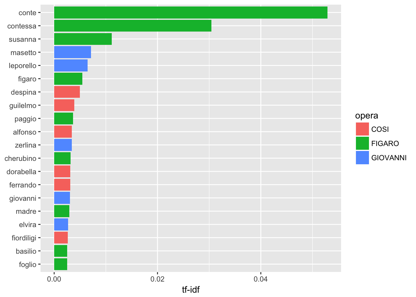
We see that character names are the most common, which makes sense! This is also similar to the results that Silge and Robinson find in their analysis of Jane Austen’s novels.
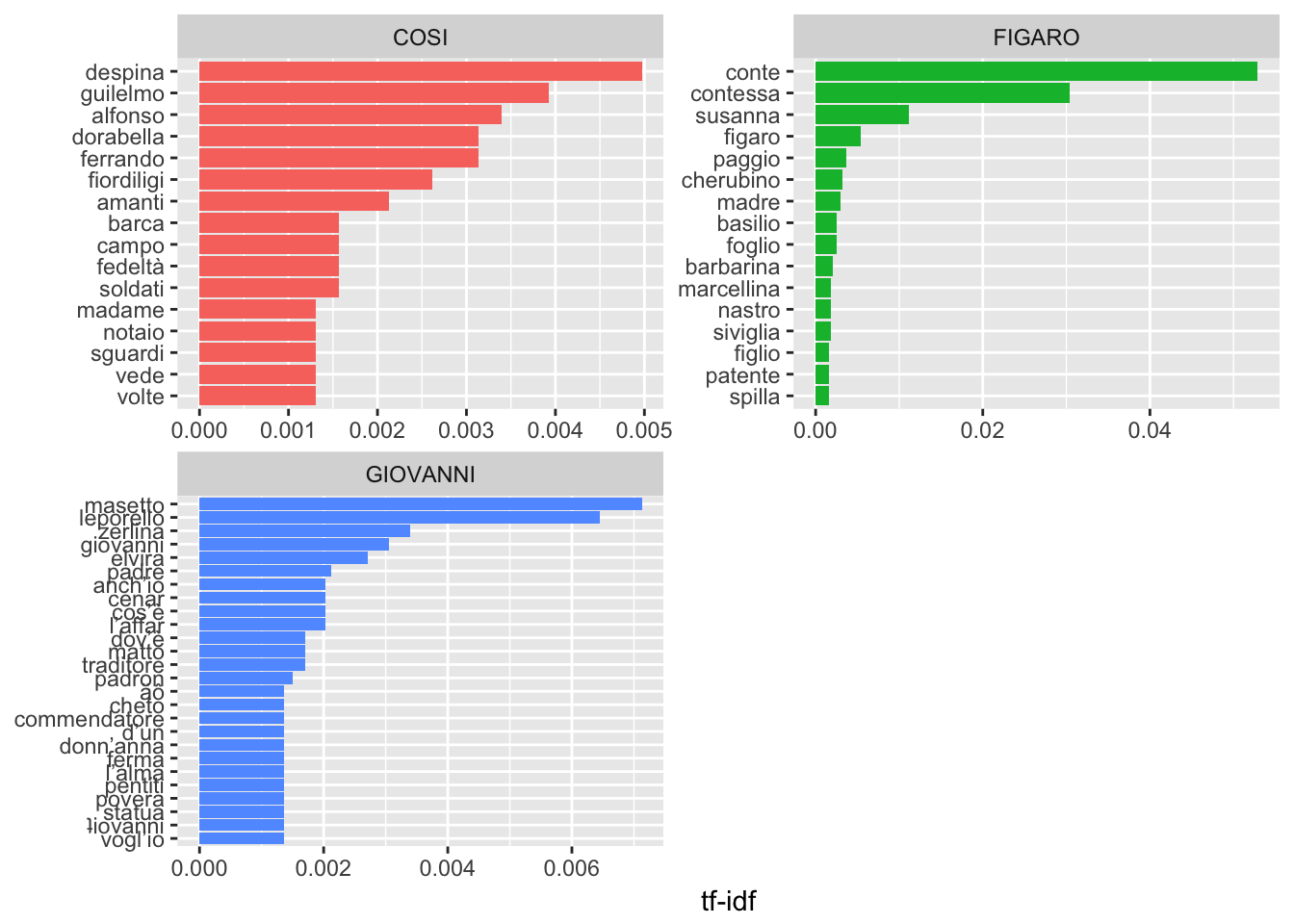
# Plot these individually
plot_mozart %>%
  group_by(opera) %>%
  top_n(15) %>%
  ungroup %>%
  ggplot(aes(word, tf_idf, fill = opera)) +
  geom_col(show.legend = FALSE) +
  labs(x = NULL, y = "tf-idf") +
  facet_wrap(~opera, ncol = 2, scales = "free") +
  coord_flip()