Twitter + Geographic Analyses

First we will look at some Twitter data of the Wicker Park neighborhood in Chicago, IL.

# key = "YOUR KEY HERE"
# secret = "YOUR SECRET HERE"

# tok = "YOUR TOK HERE"
# tok_sec = "YOUR TOK_SEC HERE"

# twitter_oauth <- setup_twitter_oauth(key, secret, tok, tok_sec)

If you don’t have the Twitter API set up, you can access the data in R data format here. If you get the data this way, start from the ‘twListToDF’ step.

Now you have set up your ‘handshake’ with the API and are ready to collect data. We will search by coordinate for all tweets that have occurred within a 1 kilometer radius of a central point in the Wicker Park neighborhood in Chicago, IL.

# geo <- searchTwitter('',n=7000,geocode='41.908602,-87.677417,1km',retryOnRateLimit=1)
# Save tweet data (if you want)
# save(geo,file=paste("sampletweetdata.Rda"))

# If you need to load that data (make sure you are in the right directory)
load('sampletweetdata.Rda')

# Convert to data frame
geoDF<-twListToDF(geo)

Now we have a data frame. We will now identify emojis, select just those tweets that come from Instagram and clean this data (get rid of links, special characters, etc.) so we can do text analyses. You can access the emoji dictionary here. The code for cleaning the tweets comes from Silge and Robinson’s book – this is special and awesome code to do this because it keeps hashtags and @ mentions. Other methods of cleaning text will count ‘#’ and ‘@’ as special characters and will get rid of them.

# Convert the encoding so you can identify emojis
geoDF$text <- iconv(geoDF$text, from = "latin1", to = "ascii", sub = "byte")

# Load in emoji dictionary. The 'trim_ws' argument is super important -- you need those spaces so the emojis aren't all squished together!
# emojis <- read_csv("Emoji Dictionary 2.1.csv", col_names=TRUE, trim_ws=FALSE)
# If you don't get weird encoding issue just use read.csv
emojis <- read.csv("Emoji Dictionary 5.0.csv", header=T)


# Go through and identify emojis
geodata <- FindReplace(data = geoDF, Var = "text", 
                            replaceData = emojis,
                       from = "R_Encoding", to = "Name", 
                       exact = FALSE)

# Just keep those tweets that come from Instagram
wicker <- geodata[geodata$statusSource == 
        "<a href=\"http://instagram.com\" rel=\"nofollow\">Instagram</a>", ]

# Get rid of stuff particular to the data (here encodings of links and such)
# Most of these are characters I don't have encodings for (other scripts, etc.)
wicker$text = gsub("Just posted a photo","", wicker$text)
wicker$text = gsub( "<.*?>", "", wicker$text)

# Now time to clean your posts. First let's make our own list of stop words again, adding additional stop words to the tidy text stop word list from the tm package stop word list.
# This makes a larger list of stop words combining those from the tm package and tidy text -- even though the tm package stop word list is pretty small anyway, just doing this just in case
data(stop_words)
mystopwords <- c(stopwords('english'),stop_words$word, "im")

# Now for Silge and Robinson's code. What this is doing is getting rid of 
# URLs, re-tweets (RT) and ampersands. This also gets rid of stop words 
# without having to get rid of hashtags and @ signs by using 
# str_detect and filter! 
reg <- "([^A-Za-z_\\d#@']|'(?![A-Za-z_\\d#@]))"
tidy_wicker <- wicker %>% 
  filter(!str_detect(text, "^RT")) %>%
  mutate(text = str_replace_all(text, "https://t.co/[A-Za-z\\d]+|http://[A-Za-z\\d]+|&amp;|&lt;|&gt;|RT|https", "")) %>%
  unnest_tokens(word, text, token = "regex", pattern = reg) %>%
  filter(!word %in% mystopwords,
         str_detect(word, "[a-z]"))

Now we have cleaned posts in tidy format. Let’s adapt some of Silge and Robinson’s code to look at frequent terms and then map concentrations of frequent terms. Note how I’ve grouped these by latitude and longitude. This will help us later on when we want to group them by coordinate.

freq <- tidy_wicker %>% 
  group_by(latitude,longitude) %>% 
  count(word, sort = TRUE) %>% 
  left_join(tidy_wicker %>% 
              group_by(latitude,longitude) %>% 
              summarise(total = n())) %>%
  mutate(freq = n/total)

# Look at most frequent terms
freq

The n here is the total number of times this term has shown up, and the total is how many terms there are present in a particular coordinate.

Cool! Now we have a representation of terms, their frequency and their position. Now I might want to plot this somehow… one way would be to try to plot the most frequent terms (n > 3) (Some help on how to do this was taken from here and here). Depending on the size of your data set, the base line for ‘most frequent’ is subject to change – because my data set is relatively small, I’m just going to say words that appear more than three times.

freq2 <- subset(freq, n > 3) 

# Let's get a map!
# This will take a couple tries to make sure you have a nice map for your data
map <- get_map(location = 'Damen and North, Chicago, Illinois', zoom = 14)

freq2$longitude<-as.numeric(freq2$longitude)
freq2$latitude<-as.numeric(freq2$latitude)
lon <- freq2$longitude
lat <- freq2$latitude

mapPoints <- ggmap(map) + geom_jitter(alpha = 0.1, size = 2.5, width = 0.25, height = 0.25) +
  geom_label_repel(data = freq2, aes(x = lon, y = lat, label = word),size = 3) 

mapPoints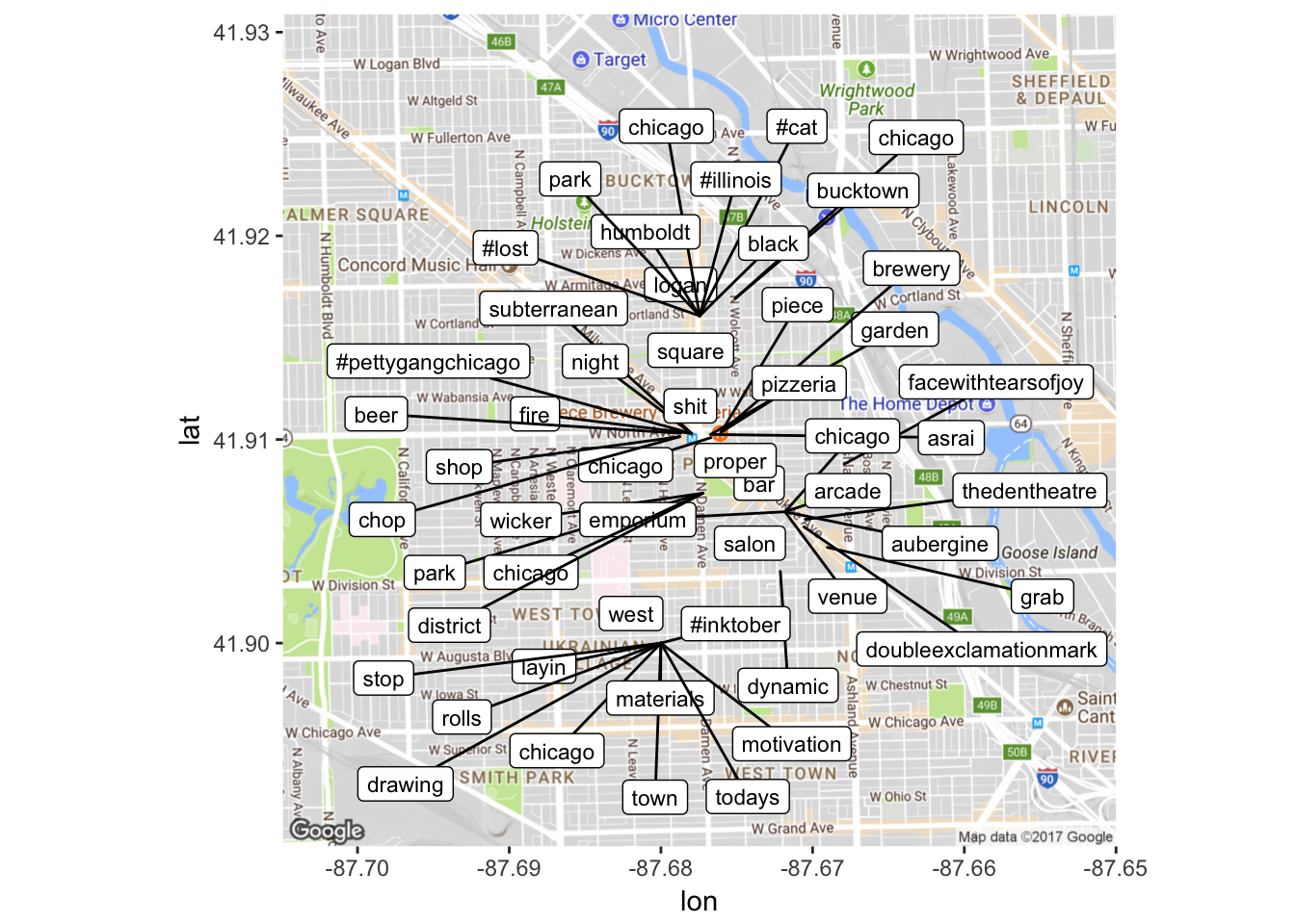

Now we have a representation of coordinates in which frequent terms are being used. A lot of these are associated with restaurants or bars (see discussion of Piece pizzeria, Emporium Arcade Bar). We can also go back and investigate certain groupings of terms – for example, the ‘#inktober’ concentration is from an artist who posts a picture of their art everyday. To check things like the concentration of ‘face with tears of joy’, we can go back to our original ‘wicker’ data frame and search for the coordinate that is in our freq2 data frame to find the links to the orginal Instagram posts or just search that coordinate on Google maps. For the coordinate where we find lots of ‘face with tears of joy’ emojis, we can see from Google maps that there is a comedy club, ‘The Comedy Clubhouse’ at that location – guess it’s a good comedy club!

How about sentiment analysis? What are the most common positive and negative words? This time we’ll just use the sentiment dictionary available in the tidytext package from the BING sentiment corpus.

# We can also look at counts of negative and positive words
bingsenti <- sentiments %>%
  filter(lexicon =="bing")

bing_word_counts <- tidy_wicker %>%
  inner_join(bingsenti) %>%
  count(word, sentiment, sort = TRUE) %>%
  ungroup()

# bing_word_counts

# Now we can graph these
# Change 'filter' parameter depending on the size of your data set
bing_word_counts %>%
  filter(n > 2) %>%
  mutate(n = ifelse(sentiment == "negative", -n, n)) %>%
  mutate(word = reorder(word, n)) %>%
  ggplot(aes(word, n, fill = sentiment)) +
  geom_bar(alpha = 0.8, stat = "identity") +
  labs(y = "Contribution to sentiment",
       x = NULL) +
  coord_flip()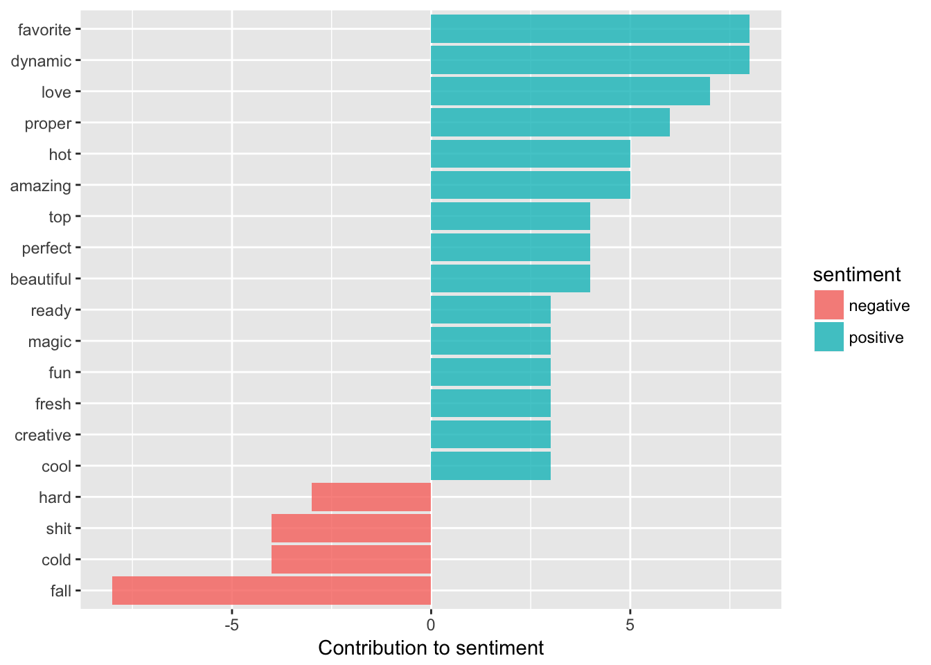

Unsurprisingly, our Instagram posts are mostly positive, with negative sentiments related to cold (Chicago!) or swear words or difficulty. We see how sentiment analysis is not always infallible, as ‘fall’ is counted as negative when really people are talking about the season and see to be happy about it.

How about a word cloud?

wordcloud(freq$word,freq$n, min.freq=3, 
          colors=brewer.pal(1, "Dark2"))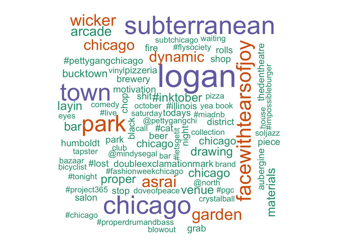

It’s interesting people talk about Logan Square a lot, but Logan Square is another neighborhood! This could be people talking about Logan Sqaure but tagging a coordinate in Wicker Park or maybe our radius was a little too big and got some Logan Square tweets (it’s pretty close). And yes, the ‘aubergine’ is the eggplant emoji. And yes, the posts are not about the vegetable.

Speaking of emojis, what are the most common emojis? What if we want to map JUST emojis? We can do this, but it involves a few steps.

# First let's 'tidy' our posts again, but DON'T make everything lowercase. This way we can isolate what are emojis and what are not emojis.
emotidy_wicker <- wicker %>%
  unnest_tokens(word, text, to_lower = FALSE)

# Let's also tidy our emoji dataframe so we can use it to filter out non-emojis in our data

emojis$Name <- as.character(emojis$Name)

tidy_emojis <- emojis %>%
  unnest_tokens(word, Name, to_lower = FALSE)

# Now we will use inner_join to keep matches and get rid of non-matches
emojis_total <- tidy_emojis %>%
  inner_join(emotidy_wicker)

# What is the most frequent emoji?
freqe <- emojis_total %>% 
   count(word, sort = TRUE)

head(freqe)

## # A tibble: 6 x 2
##                             word     n
##                            <chr> <int>
## 1             FACEWITHTEARSOFJOY    12
## 2 SMILINGFACEWITHHEARTSHAPEDEYES     6
## 3                           FIRE     5
## 4                      AUBERGINE     4
## 5          DOUBLEEXCLAMATIONMARK     4
## 6                           EYES     4

# Now we have our most common emojis. Note skin color is not separate -- you can go into the CSV file to change this if you want.

# Map it
# left_join to keep all instances, not just one
test <- freqe %>%
  left_join(emojis_total, freqe, by = "word")

# Get rid of duplicates
freqe2 <- subset(test, n > 3) 
# Get rid of duplicates
freqe2 <- freqe2[!duplicated(freqe2$id),]

freqe2$longitude<-as.numeric(freqe2$longitude)
freqe2$latitude<-as.numeric(freqe2$latitude)

mapPoints2 <- ggmap(map) + geom_jitter(alpha = 0.1, size = 2.5, width = 0.25, height = 0.25) +
  geom_label_repel(data = freqe2, aes(x = longitude, y = latitude, label = word),size = 3) 

mapPoints2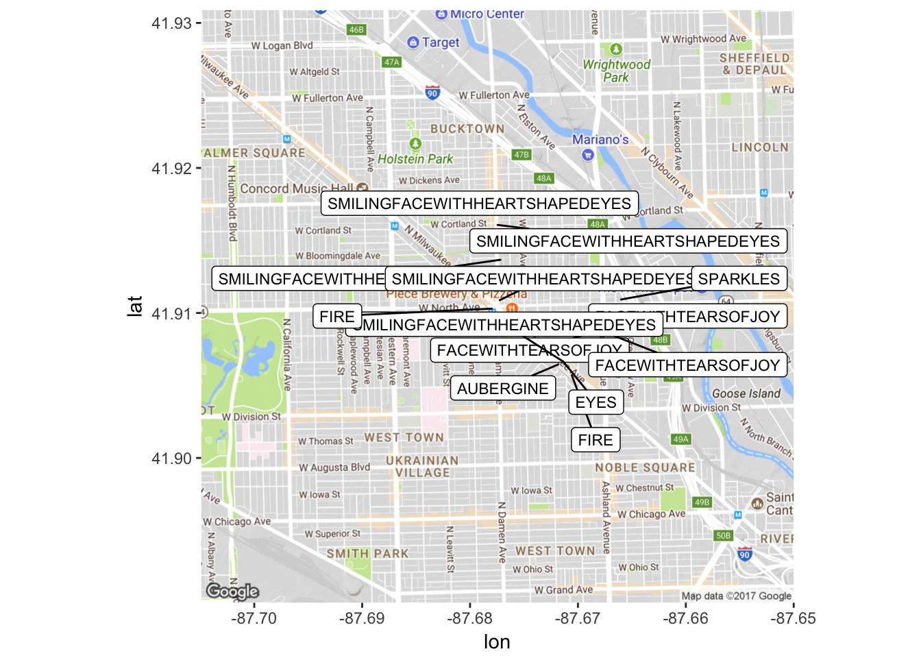

This is more impressive with a larger data set, but you can see the kinds of things you can look at with these tools. Let’s look at another visualization technique, actually graphing with emojis using the ‘emoGG’ package. Once again, this takes a few steps to set up.

Let’s do the top six: 😂 😍 🔥 🍆 ✨ and 👀.

# We will use emoGG to find the right code for each one. You can cross-check this with the unicode codepoint listed in your emoji dictionary (usualy they are the same, with all letters in lowercase).
# How to search:
# Identifier for each one for mapping
# 'face with tears of joy' 1f602
# 'heart eyes' 1f60d
# 'fire' 1f525
# 'aubergine' 1f346
# 'sparkles' 2728
# 'eyes' 1f440

tearsofjoygrep <- grepl(paste("FACEWITHTEARSOFJOY"), freqe2$word)
tearsofjoyDF<-as.data.frame(tearsofjoygrep)
freqe2$ID7 <- 1:nrow(freqe2)
tearsofjoyDF$ID7 <- 1:nrow(tearsofjoyDF)
freqe2 <- merge(freqe2,tearsofjoyDF,by="ID7")
tearsofjoy <- freqe2[freqe2$tearsofjoygrep == "TRUE", ]

sparkgrep <- grepl(paste("SPARKLES"), freqe2$word)
sparkDF<-as.data.frame(sparkgrep)
sparkDF$ID7 <- 1:nrow(sparkDF)
freqe2 <- merge(freqe2,sparkDF,by="ID7")
spark <- freqe2[freqe2$sparkgrep == "TRUE", ]

egggrep <- grepl(paste("AUBERGINE"), freqe2$word)
eggDF <-as.data.frame(egggrep)
eggDF$ID7 <- 1:nrow(eggDF)
freqe2 <- merge(freqe2,eggDF,by="ID7")
aubergine <- freqe2[freqe2$egggrep == "TRUE", ]

firegrep <- grepl(paste("FIRE"), freqe2$word)
fireDF<-as.data.frame(firegrep)
fireDF$ID7 <- 1:nrow(fireDF)
freqe2 <- merge(freqe2,fireDF,by="ID7")
fire <- freqe2[freqe2$firegrep == "TRUE", ]

eyesgrep <- grepl(paste("EYES"), freqe2$word)
eyesDF<-as.data.frame(eyesgrep)
eyesDF$ID7 <- 1:nrow(eyesDF)
freqe2 <- merge(freqe2,eyesDF,by="ID7")
eyes <- freqe2[freqe2$eyesgrep == "TRUE", ]

heartgrep <- grepl(paste("SMILINGFACEWITHHEARTSHAPEDEYES"), freqe2$word)
heartDF<-as.data.frame(heartgrep)
heartDF$ID7 <- 1:nrow(heartDF)
freqe2 <- merge(freqe2,heartDF,by="ID7")
hearteyes <- freqe2[freqe2$heartgrep == "TRUE", ]


# Map this
# Some stuff we have to do first
tearsofjoy$latitude <- as.numeric(tearsofjoy$latitude)
tearsofjoy$longitude <- as.numeric(tearsofjoy$longitude)
spark$latitude <- as.numeric(spark$latitude)
spark$longitude <- as.numeric(spark$longitude)
aubergine$latitude <- as.numeric(aubergine$latitude)
aubergine$longitude <- as.numeric(aubergine$longitude)
fire$latitude <- as.numeric(fire$latitude)
fire$longitude <- as.numeric(fire$longitude)
eyes$latitude <- as.numeric(eyes$latitude)
eyes$longitude <- as.numeric(eyes$longitude)
hearteyes$latitude <- as.numeric(hearteyes$latitude)
hearteyes$longitude <- as.numeric(hearteyes$longitude)

# Get a new map that is zoomed in a bit more
map2 <- get_map(location = 'Damen and North, Chicago, Illinois', zoom = 15)


emomap <- ggmap(map2) + geom_emoji(aes(x = longitude, y = latitude), 
                                     data=tearsofjoy, emoji="1f602") +
                              geom_emoji(aes(x=longitude, y=latitude),
                                     data=spark, emoji="2728") +
                              geom_emoji(aes(x=longitude, y=latitude),
                                     data=aubergine, emoji="1f346") +
                              geom_emoji(aes(x=longitude, y=latitude),
                                     data=fire, emoji="1f525") +
                              geom_emoji(aes(x=longitude, y=latitude),
                                     data=eyes, emoji="1f440") +
                              geom_emoji(aes(x=longitude, y=latitude),
                                     data=hearteyes, emoji="1f60d")

emomap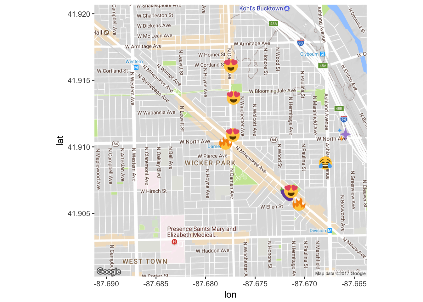

Again, this is more impressive when you have more data. You can see some examples of this here.

YouTube + Diachronic Sentiment Analysis

Onwards to YouTube data! We’ll be doing some similar analyses, like sentiment analysis, but instead of looking at things in terms of coordinates, we’ll look at things in terms of time. I wanted to choose something that had a lot of comments, so let’s look at the comments from the ill-advised (and ill-fated) ‘Emoji Movie’ trailer. This also has a lot of varying sentiment (one of the comments is “The movie is a such disgrace to the animation film industry.”😹😹😹).

If you don’t have the YouTube API set up, you can access the data here.

# Connect to YouTube API
# Leave token blank
# yt_oauth("app_id", "app_password", token='')

 # emojimovie <- get_comment_threads(c(video_id="o_nfdzMhmrA"), max_results = 101)

# Save data (if you want)
# save(emojimovie,file=paste("sampletubedata.Rda"))

# If you need to load that data (make sure you are in the right directory)
load('sampletubedata.Rda')

Now we have some (~10,300) comments to play with. Due to the subject matter, emojis are likely to be frequent in our data set, so let’s follow the same procedure as with our tweets to identify those emojis and label them.

Help figuring out the emoji encoding issue from Patrick Perry – thanks Patrick! 😊

emojis <- read.csv('Emoji Dictionary 5.0.csv', stringsAsFactors = FALSE)
# change U+1F469 U+200D U+1F467 to \U1F469\U200D\U1F467
emojis$escapes <- gsub("[[:space:]]*\\U\\+", "\\\\U", emojis$Codepoint)

# convert to UTF-8 using the R parser
emojis$codes <- sapply(parse(text = paste0("'", emojis$escapes, "'"),
                      keep.source = FALSE), eval)

emojimovie$text <- as.character(emojimovie$textOriginal)

# Go through and identify emojis
emoemo <- FindReplace(data = emojimovie, Var = "text", 
                            replaceData = emojis,
                       from = "codes", to = "Name", 
                       exact = FALSE)
# This might take some time, we have a big data set. 

Now let’s clean our data using the same code as we used for our tweets (in case there are any hashtags or @ mentions).

emoemo$text = gsub( "<.*?>", "", emoemo$text)

reg <- "([^A-Za-z_\\d#@']|'(?![A-Za-z_\\d#@]))"
tidy_tube <- emoemo %>% 
  filter(!str_detect(text, "^RT")) %>%
  mutate(text = str_replace_all(text, "https://t.co/[A-Za-z\\d]+|http://[A-Za-z\\d]+|&amp;|&lt;|&gt;|RT|https", "")) %>%
  unnest_tokens(word, text, token = "regex", pattern = reg) %>%
  filter(!word %in% mystopwords,
         str_detect(word, "[a-z]"))

freqtube <- tidy_tube %>% 
  group_by(publishedAt) %>% 
  count(word, sort = TRUE) %>% 
  left_join(tidy_tube %>% 
              group_by(publishedAt) %>% 
              summarise(total = n())) %>%
  mutate(freq = n/total)

# Look at most frequent terms
head(freqtube)

## # A tibble: 6 x 5
## # Groups:   publishedAt [5]
##                publishedAt               word     n total       freq
##                     <fctr>              <chr> <int> <int>      <dbl>
## 1 2017-10-23T13:00:06.000Z facewithtearsofjoy  2163  2163 1.00000000
## 2 2017-10-12T11:42:22.000Z          pileofpoo   412  1133 0.36363636
## 3 2017-10-07T07:49:00.000Z facewithtearsofjoy   309  1133 0.27272727
## 4 2017-10-15T21:17:26.000Z               film   309  3708 0.08333333
## 5 2017-10-06T18:22:11.000Z              cheap   206   927 0.22222222
## 6 2017-10-06T18:22:11.000Z              knock   206   927 0.22222222

bing_word_countstube <- tidy_tube %>%
  inner_join(bingsenti) %>%
  count(word, sentiment, sort = TRUE) %>%
  ungroup()

# bing_word_counts

# Now we can graph these
# Change 'filter' parameter depending on the size of your data set
bing_word_countstube %>%
  filter(n > 100) %>%
  mutate(n = ifelse(sentiment == "negative", -n, n)) %>%
  mutate(word = reorder(word, n)) %>%
  ggplot(aes(word, n, fill = sentiment)) +
  geom_bar(alpha = 0.8, stat = "identity") +
  labs(y = "Contribution to sentiment",
       x = NULL) +
  coord_flip()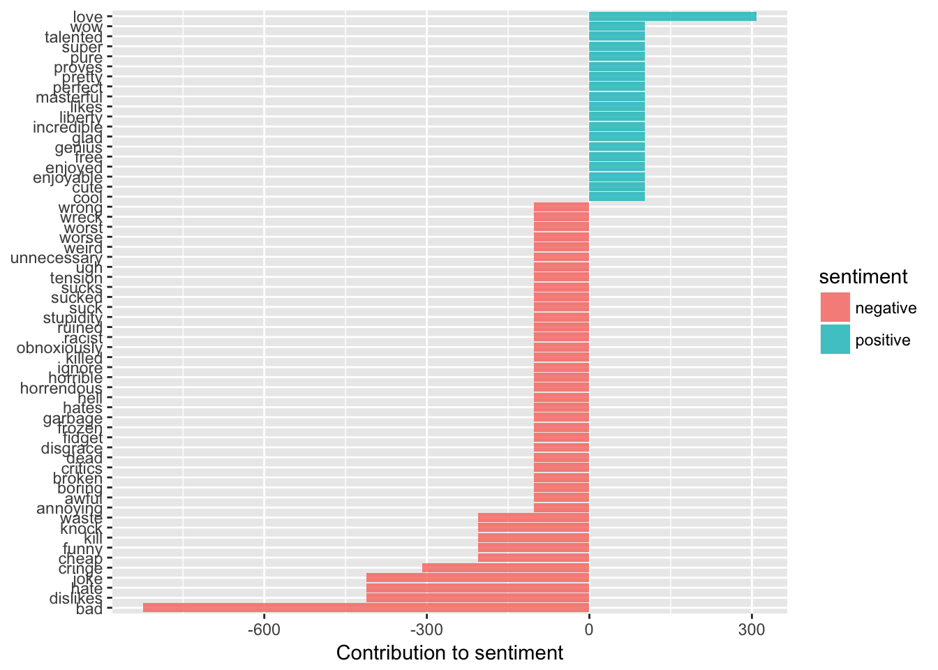

Perhaps unsurprisingly, it seems most of our comments are negative. We can see here some of the biggest contributors to negative sentiment, terms like ‘disgrace’ or ‘hate’, ‘cheap’ or ‘cringe’.

Let’s look at things over time. Code from Silge and Robinson. This example is looking at the words that have changed the most over time in terms of frequency.

# Need to change some formatting
tidy_tube$created <- as.character(tidy_tube$publishedAt)
tidy_tube$created <- as.POSIXct(tidy_tube$created)

words_by_time <- tidy_tube %>%
  filter(!str_detect(word, "^@")) %>%
  mutate(time_floor = floor_date(created, unit = "1 day")) %>%
  count(time_floor, word) %>%
  ungroup() %>%
  group_by(time_floor) %>%
  mutate(time_total = sum(n)) %>%
  group_by(word) %>%
  mutate(word_total = sum(n)) %>%
  ungroup() %>%
  rename(count = n) %>%
  filter(word_total > 300)

# words_by_time
nested_data <- words_by_time %>%
  nest(-word) 

# nested_data

nested_models <- nested_data %>%
  mutate(models = map(data, ~ glm(cbind(count, time_total) ~ time_floor, ., 
                                  family = "binomial")))

# nested_models


slopes <- nested_models %>%
  unnest(map(models, tidy)) %>%
  filter(term == "time_floor") %>%
  mutate(adjusted.p.value = p.adjust(p.value))

top_slopes <- slopes %>% 
  filter(adjusted.p.value < 0.1)

# top_slopes

# Graph
words_by_time %>%
  inner_join(top_slopes, by = c("word")) %>%
  ggplot(aes(time_floor, count/time_total, color = word)) +
  geom_line(size = 1.3) +
  labs(x = NULL, y = "Word frequency")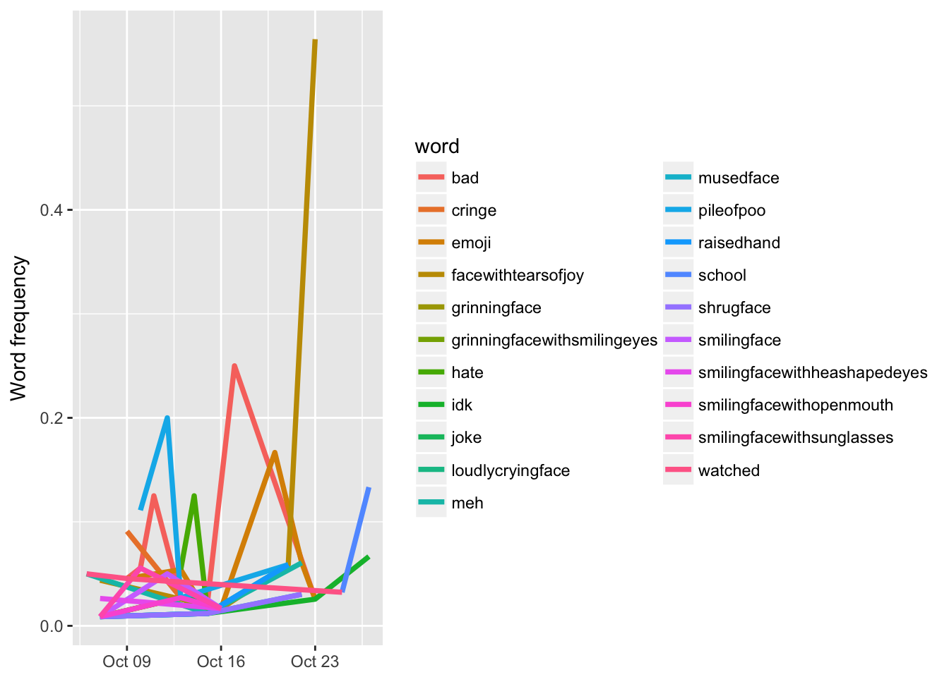

# Graph a subset of just slopes of emojis
# Have to make them lowercase for this 
emojis2 <- emojis %>%
  unnest_tokens(word, Name)

sub_slopes <- top_slopes %>%
  inner_join(emojis2)
  
  
words_by_time %>%
  inner_join(sub_slopes, by = c("word")) %>%
  ggplot(aes(time_floor, count/time_total, color = word)) +
  geom_line(size = 1.3) +
  labs(x = NULL, y = "Word frequency")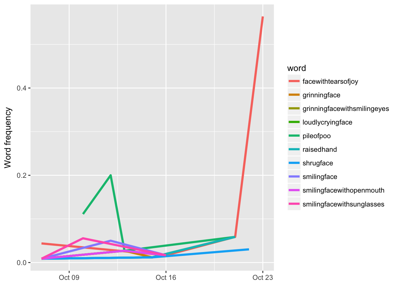

What are the most common emojis in comments about the emoji movie?

# Same steps as above
emotidy_tube <- emoemo %>%
  unnest_tokens(word, text, to_lower = FALSE)

emojis$Name <- as.character(emojis$Name)
tube_tidy_emojis <- emojis %>%
  unnest_tokens(word, Name, to_lower = FALSE)

# Now we will use inner_join to keep matches and get rid of non-matches
tube_emojis_total <- tube_tidy_emojis %>%
  inner_join(emotidy_tube)

# What is the most frequent emoji?
tube_freqe <- tube_emojis_total %>% 
   count(word, sort = TRUE)

head(tube_freqe)

## # A tibble: 6 x 2
##                             word     n
##                            <chr> <int>
## 1             FACEWITHTEARSOFJOY  2987
## 2                      PILEOFPOO   824
## 3                   GRINNINGFACE   412
## 4 SMILINGFACEWITHHEARTSHAPEDEYES   412
## 5                      AUBERGINE   309
## 6    GRINNINGFACEWITHSMILINGEYES   309

So, our most frequent emojis in the comments of the Emoji Movie trailer are 😂, 💩, 😀, 😍, 😁 and 🍆. Read into that what you will! 😂